Case study for tidyMass
Hong Yan (https://ysph.yale.edu/profile/hong_yan/)
Xiaotao Shen (https://www.shenxt.info/)
Chuhu Wang (https://www.linkedin.com/in/chuchu-wang-71331190/)
Created on 2022-03-03 and updated on 2022-03-09
tidymass_case_study.RmdIntroduction
Data introduction. We have RPLC (positive and negative mode), HILIC (positive and negative mode). More information can be found here.
Sex Differences in Colon Cancer Metabolism Reveal A Novel Subphenotype
Download data
Mass spectrometry raw data (mzXML) for the case study in this paper is accessible on MetaboLights with MTBLS1122 (HILIC positive), MTBLS1124 (HILIC negative), MTBLS1122 (RPLC positive) and MTBLS1130 (RPLC negative). The MS2 data (mgf) and processed data (“mass_dataset” class) from the massProcesser package are available on the tidyMass project website (https://tidymass.github.io/case_study_data/).
Note: In some steps, we just skip them to save time, try to change
eval=FALSEtoeval=TRUEso you can run this code chunk. For the annotation step, because we can’t share the in-house database, so we just provide themass_datasetclass after annotation. We apologize for the inconvenience.
Data preparation
Please download all the data and code, and put them in one folder named as case_study.

Install packages
Please install the pacakge we need in this analysis.
tidymass
Please refer this document.
if(!require(remotes)){
install.packages("remotes")
}
if(!require(remotes)){
remotes::install_gitlab("jaspershen/tidymass")
}
tidyverse
if(!require(tidyverse)){
install.packages("tidyverse")
}Other packages
if(!require(BiocManager)){
install.packages("BiocManager")
}
if(!require(ComplexHeatmap)){
BiocManager::install("ComplexHeatmap")
}
if(!require(ggraph)){
install.packages("ggraph")
}
if(!require(tidygraph)){
install.packages("tidygraph")
}
if(!require(extrafont)){
install.packages("extrafont")
}
if(!require(shadowtext)){
install.packages("shadowtext")
}Raw data processing
massprocesser package is used to do the raw data processing. Please refer this website for more information.
RPLC positive mode
The code used to do raw data processing.
process_data(
path = "mzxml_ms1_data/RPLC/POS/",
polarity = "positive",
ppm = 20,
peakwidth = c(5, 30),
threads = 6,
output_tic = FALSE,
output_bpc = FALSE,
output_rt_correction_plot = FALSE,
min_fraction = 0.5,
group_for_figure = "QC"
)All the results will be placed in the folder named case_study/data/mzxml_ms1_data/POS/Result. More information about that can be found here.
You can just load the object, which is a mass_dataset class object.
load("mzxml_ms1_data/RPLC/POS/Result/object")
object
#> --------------------
#> massdataset version: 0.99.9
#> --------------------
#> 1.expression_data:[ 14585 x 298 data.frame]
#> 2.sample_info:[ 298 x 4 data.frame]
#> 3.variable_info:[ 14585 x 3 data.frame]
#> 4.sample_info_note:[ 4 x 2 data.frame]
#> 5.variable_info_note:[ 3 x 2 data.frame]
#> 6.ms2_data:[ 0 variables x 0 MS2 spectra]
#> --------------------
#> Processing information (extract_process_info())
#> create_mass_dataset ----------
#> Package Function.used Time
#> 1 massdataset create_mass_dataset() 2022-03-02 14:50:02
#> process_data ----------
#> Package Function.used Time
#> 1 massprocesser process_data 2022-03-02 12:25:08
dim(object)
#> [1] 14585 298We can see that there are 14,585 metabolic features in positive mode.
RT correction plot
load data
load("mzxml_ms1_data/RPLC/POS/Result/intermediate_data/xdata2")Set the group_for_figure if you want to show specific groups. And set it as “all” if you want to show all samples.
We can use the plot_adjusted_rt() function to get the interactive plot.
load("mzxml_ms1_data/RPLC/POS/Result/intermediate_data/xdata2")
####set the group_for_figure if you want to show specific groups.
####And set it as "all" if you want to show all samples.
plot <-
massprocesser::plot_adjusted_rt(object = xdata2,
group_for_figure = "QC",
interactive = TRUE)
plotRPLC negative mode
The processing of negative mode is same with positive mode data.
Same with positive mode, change polarity to negative.
process_data(
path = "mzxml_ms1_data/RPLC/NEG/",
polarity = "negative",
ppm = 20,
peakwidth = c(5, 30),
threads = 6,
output_tic = FALSE,
output_bpc = FALSE,
output_rt_correction_plot = FALSE,
min_fraction = 0.5,
group_for_figure = "QC"
)Same with positive mode.
load("mzxml_ms1_data/RPLC/NEG/Result/object")
object
#> --------------------
#> massdataset version: 0.99.2
#> --------------------
#> 1.expression_data:[ 4685 x 299 data.frame]
#> 2.sample_info:[ 299 x 4 data.frame]
#> 3.variable_info:[ 4685 x 3 data.frame]
#> 4.sample_info_note:[ 4 x 2 data.frame]
#> 5.variable_info_note:[ 3 x 2 data.frame]
#> 6.ms2_data:[ 0 variables x 0 MS2 spectra]
#> --------------------
#> Processing information (extract_process_info())
#> create_mass_dataset ----------
#> Package Function.used Time
#> 1 massdataset create_mass_dataset() 2022-03-01 09:51:34
#> process_data ----------
#> Package Function.used Time
#> 1 massprocesser process_data 2022-03-01 09:03:10
dim(object)
#> [1] 4685 299We can see that there are 4,685 metabolic features in negative mode.
HILIC positive mode
process_data(
path = "mzxml_ms1_data/HILIC/POS/",
polarity = "positive",
ppm = 20,
peakwidth = c(5, 30),
threads = 6,
output_tic = FALSE,
output_bpc = FALSE,
output_rt_correction_plot = FALSE,
min_fraction = 0.5,
group_for_figure = "QC"
)HILIC negative mode
process_data(
path = "mzxml_ms1_data/HILIC/NEG/",
polarity = "negative",
ppm = 20,
peakwidth = c(5, 30),
threads = 6,
output_tic = FALSE,
output_bpc = FALSE,
output_rt_correction_plot = FALSE,
min_fraction = 0.5,
group_for_figure = "QC"
)Explore data
After the raw data processing, peak tables for positive and negative mode will be generated.
RPLC positive mode
load("mzxml_ms1_data/RPLC/POS/Result/object")
object_rplc_pos <- object
object_rplc_pos
#> --------------------
#> massdataset version: 0.99.9
#> --------------------
#> 1.expression_data:[ 14585 x 298 data.frame]
#> 2.sample_info:[ 298 x 4 data.frame]
#> 3.variable_info:[ 14585 x 3 data.frame]
#> 4.sample_info_note:[ 4 x 2 data.frame]
#> 5.variable_info_note:[ 3 x 2 data.frame]
#> 6.ms2_data:[ 0 variables x 0 MS2 spectra]
#> --------------------
#> Processing information (extract_process_info())
#> create_mass_dataset ----------
#> Package Function.used Time
#> 1 massdataset create_mass_dataset() 2022-03-02 14:50:02
#> process_data ----------
#> Package Function.used Time
#> 1 massprocesser process_data 2022-03-02 12:25:08Read sample information.
sample_info_pos <-
readr::read_csv("sample_info/RPLC/sample_info_pos_1.csv")
#> Rows: 299 Columns: 6
#> ── Column specification ────────────────────────────────────────────────────────
#> Delimiter: ","
#> chr (4): sample_id, class, subject_id, group
#> dbl (2): injection.order, batch
#>
#> ℹ Use `spec()` to retrieve the full column specification for this data.
#> ℹ Specify the column types or set `show_col_types = FALSE` to quiet this message.
head(sample_info_pos)
#> # A tibble: 6 × 6
#> sample_id injection.order class batch subject_id group
#> <chr> <dbl> <chr> <dbl> <chr> <chr>
#> 1 men_normal_166 21 control 1 men_normal_166 male control
#> 2 men_normal_2332 220 control 1 men_normal_2332 male control
#> 3 men_normal_2357 222 control 1 men_normal_2357 male control
#> 4 men_normal_2371 223 control 1 men_normal_2371 male control
#> 5 men_normal_2407 224 control 1 men_normal_2407 male control
#> 6 men_normal_2409 226 control 1 men_normal_2409 male controlAdd sample_info_pos to object_rplc_pos
object_rplc_pos %>%
extract_sample_info() %>%
head()
#> sample_id group class injection.order
#> 1 men_normal_166 Case Subject 1
#> 2 men_normal_2332 Case Subject 2
#> 3 men_normal_2357 Case Subject 3
#> 4 men_normal_2371 Case Subject 4
#> 5 men_normal_2407 Case Subject 5
#> 6 men_normal_2409 Case Subject 6
object_rplc_pos <-
object_rplc_pos %>%
activate_mass_dataset(what = "sample_info") %>%
dplyr::select(-c(group, class, injection.order))
object_rplc_pos <-
object_rplc_pos %>%
activate_mass_dataset(what = "sample_info") %>%
left_join(sample_info_pos,
by = "sample_id")
object_rplc_pos %>%
extract_sample_info() %>%
head()
#> sample_id injection.order class batch subject_id group
#> 1 men_normal_166 21 control 1 men_normal_166 male control
#> 2 men_normal_2332 220 control 1 men_normal_2332 male control
#> 3 men_normal_2357 222 control 1 men_normal_2357 male control
#> 4 men_normal_2371 223 control 1 men_normal_2371 male control
#> 5 men_normal_2407 224 control 1 men_normal_2407 male control
#> 6 men_normal_2409 226 control 1 men_normal_2409 male control
dim(object_rplc_pos)
#> [1] 14585 298
object_rplc_pos %>%
activate_mass_dataset(what = "sample_info") %>%
dplyr::count(class)
#> class n
#> 1 case 228
#> 2 control 42
#> 3 QC 28
object_rplc_pos %>%
activate_mass_dataset(what = "sample_info") %>%
dplyr::count(group)
#> group n
#> 1 female control 14
#> 2 female LCC 50
#> 3 female RCC 60
#> 4 male control 28
#> 5 male LCC 63
#> 6 male RCC 55
#> 7 QC 28
object_rplc_pos %>%
activate_mass_dataset(what = "sample_info") %>%
dplyr::count(batch)
#> batch n
#> 1 1 298Next, we can get the peak distributation plot of positive mode.
object_rplc_pos %>%
`+`(1) %>%
log(10) %>%
show_mz_rt_plot() +
scale_size_continuous(range = c(0.01, 2))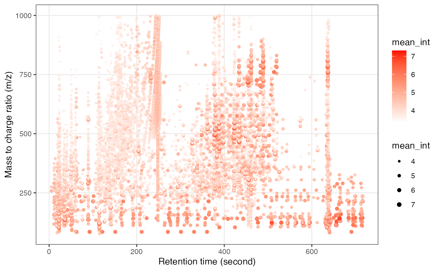
We can explore the missing values in positive mode data.
get_mv_number(object = object_rplc_pos)
#> [1] 1920550Missing value number in each sample.
get_mv_number(object = object_rplc_pos, by = "variable") %>%
head()
#> M77T115_POS M82T641_POS M82T18_POS M84T22_POS M84T19_POS M85T92_POS
#> 47 149 103 116 159 70Missing value number in each variable.
We can use the figure to show the missing value information.
library(grid)
show_missing_values(object = object_rplc_pos,
show_column_names = FALSE,
percentage = TRUE)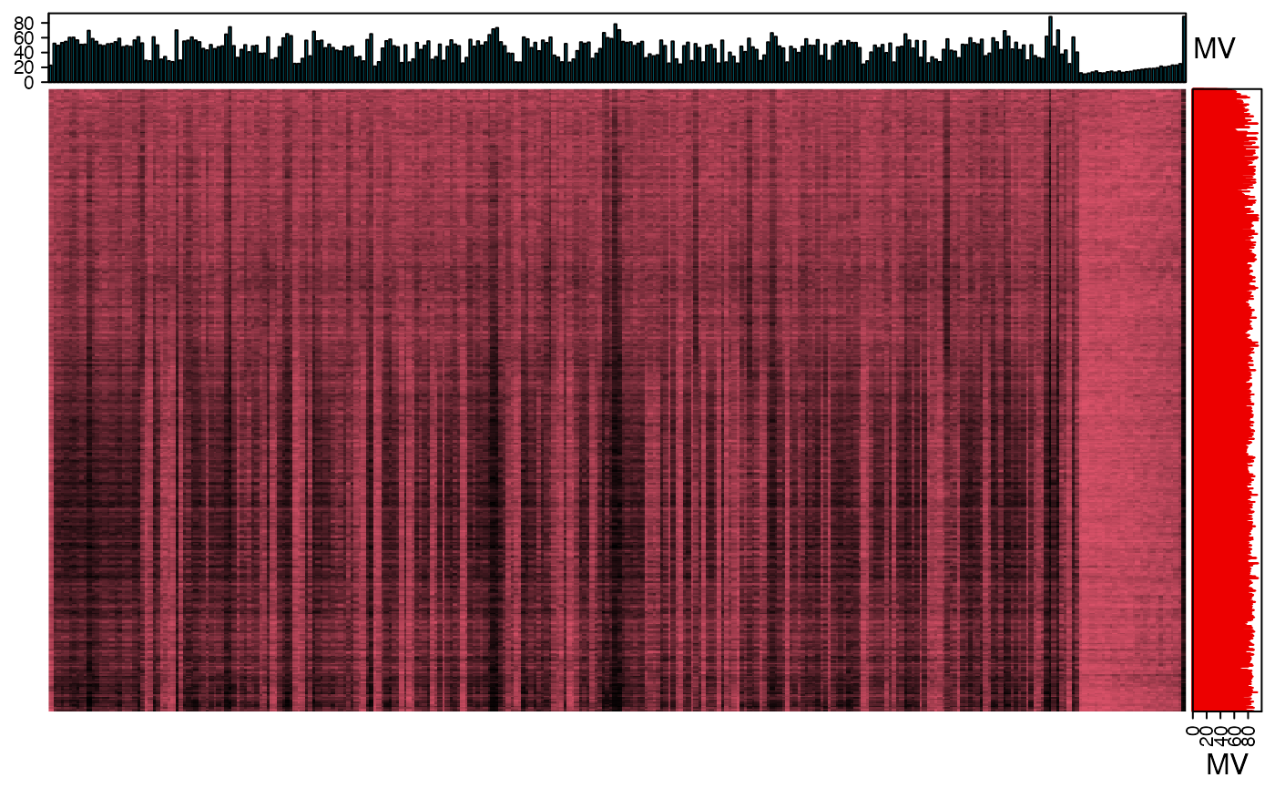
Show the mvs in samples.
show_sample_missing_values(object = object_rplc_pos,
percentage = TRUE) +
scale_size_continuous(range = c(0.1, 1)) +
theme(axis.text.x = element_blank(),
axis.ticks.x = element_blank())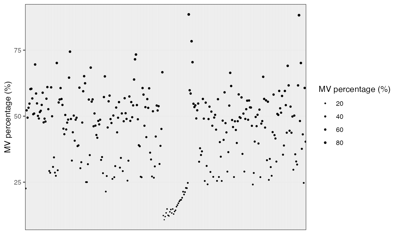
Show the mvs in variables
show_variable_missing_values(object = object_rplc_pos,
percentage = TRUE,
show_x_text = FALSE,
show_x_ticks = FALSE) +
scale_size_continuous(range = c(0.01, 1))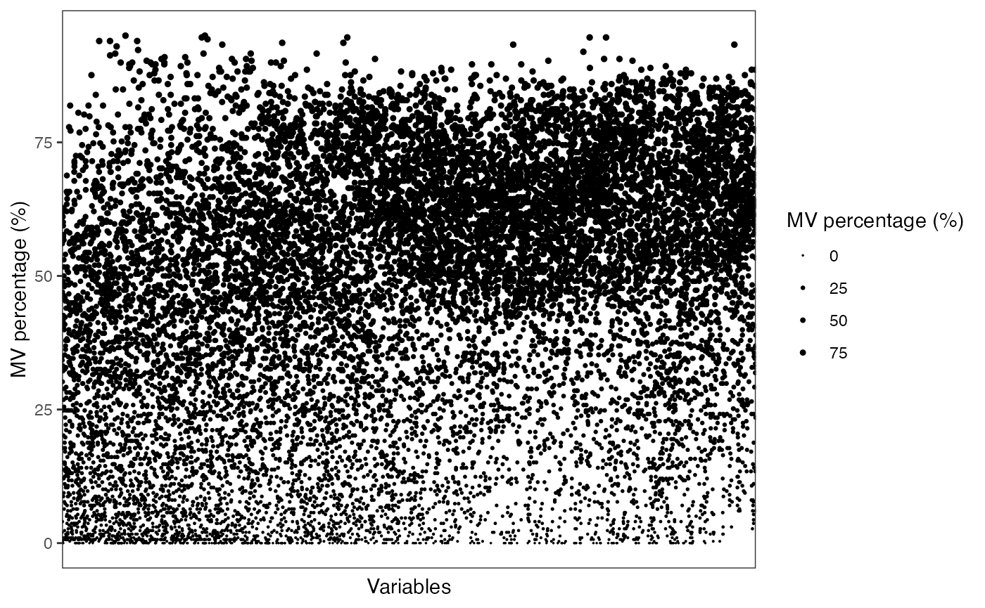
RPLC Negative mode
Load object.
load("mzxml_ms1_data/RPLC/NEG/Result/object")
object_rplc_neg <- object
object_rplc_neg
#> --------------------
#> massdataset version: 0.99.2
#> --------------------
#> 1.expression_data:[ 4685 x 299 data.frame]
#> 2.sample_info:[ 299 x 4 data.frame]
#> 3.variable_info:[ 4685 x 3 data.frame]
#> 4.sample_info_note:[ 4 x 2 data.frame]
#> 5.variable_info_note:[ 3 x 2 data.frame]
#> 6.ms2_data:[ 0 variables x 0 MS2 spectra]
#> --------------------
#> Processing information (extract_process_info())
#> create_mass_dataset ----------
#> Package Function.used Time
#> 1 massdataset create_mass_dataset() 2022-03-01 09:51:34
#> process_data ----------
#> Package Function.used Time
#> 1 massprocesser process_data 2022-03-01 09:03:10Read sample information.
sample_info_neg <- readr::read_csv("sample_info/RPLC/sample_info_neg_1.csv")
#> Rows: 299 Columns: 6
#> ── Column specification ────────────────────────────────────────────────────────
#> Delimiter: ","
#> chr (4): sample_id, class, subject_id, group
#> dbl (2): injection.order, batch
#>
#> ℹ Use `spec()` to retrieve the full column specification for this data.
#> ℹ Specify the column types or set `show_col_types = FALSE` to quiet this message.
head(sample_info_neg)
#> # A tibble: 6 × 6
#> sample_id injection.order class batch subject_id group
#> <chr> <dbl> <chr> <dbl> <chr> <chr>
#> 1 men_normal_166 21 control 1 men_normal_166 male control
#> 2 men_normal_2332 220 control 1 men_normal_2332 male control
#> 3 men_normal_2357 222 control 1 men_normal_2357 male control
#> 4 men_normal_2371 223 control 1 men_normal_2371 male control
#> 5 men_normal_2407 224 control 1 men_normal_2407 male control
#> 6 men_normal_2409 226 control 1 men_normal_2409 male controlAdd sample_info_neg to object_rplc_neg
object_rplc_neg <-
object_rplc_neg %>%
activate_mass_dataset(what = "sample_info") %>%
dplyr::select(-c("group", "class", "injection.order"))
object_rplc_neg <-
object_rplc_neg %>%
activate_mass_dataset(what = "sample_info") %>%
left_join(sample_info_neg,
by = "sample_id")Next, we can get the peak distributation plot of negative mode.
object_rplc_neg %>%
`+`(1) %>%
log(10) %>%
show_mz_rt_plot() +
scale_size_continuous(range = c(0.01, 2))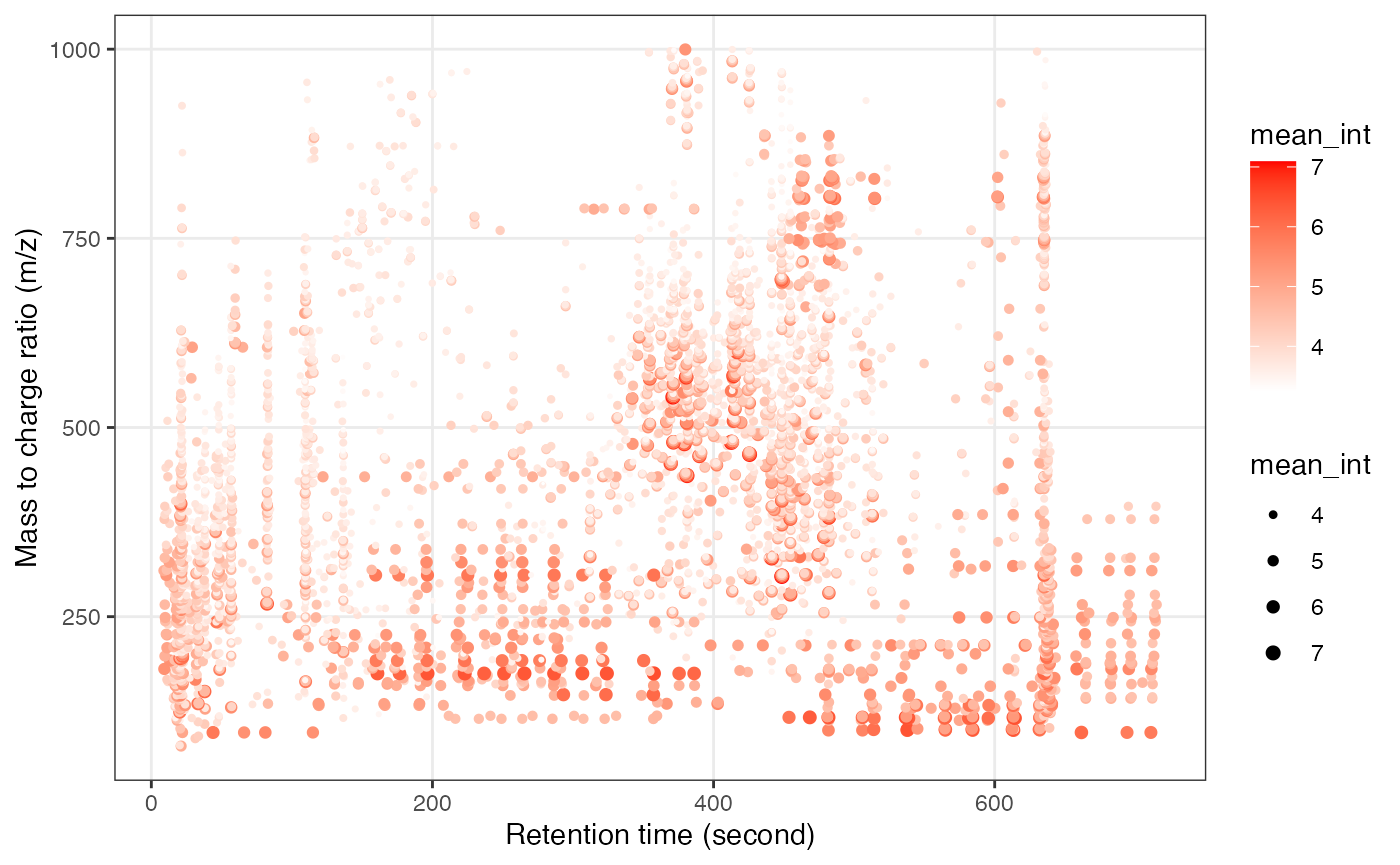
We can explore the missing values in negative mode data.
We can use the figure to show the missing value information.
show_missing_values(object = object_rplc_neg, show_column_names = FALSE, percentage = TRUE)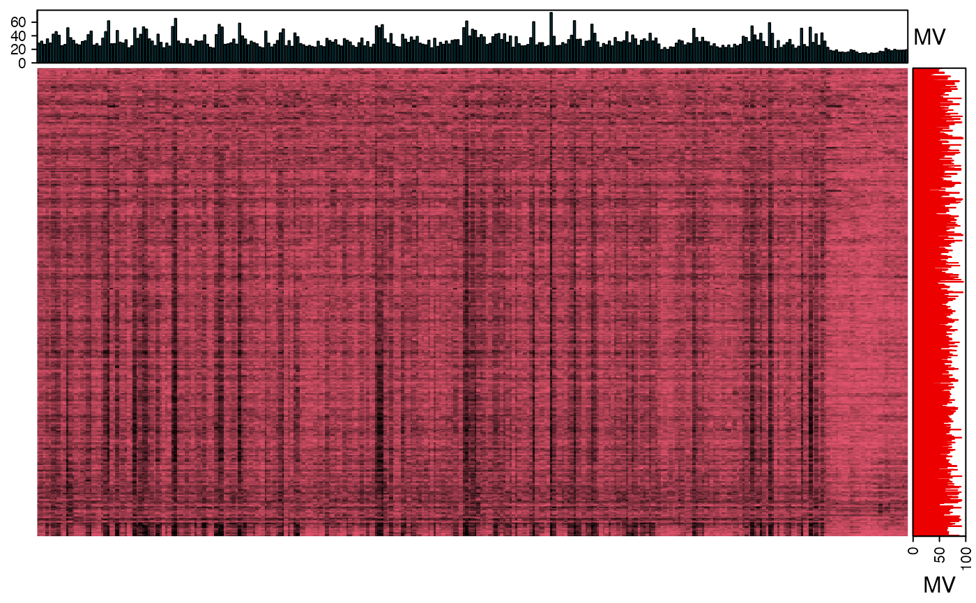
HILIC positive mode
load("mzxml_ms1_data/HILIC/POS/Result/object")
object_hilic_pos <- object
object_hilic_pos
#> --------------------
#> massdataset version: 0.99.9
#> --------------------
#> 1.expression_data:[ 5322 x 299 data.frame]
#> 2.sample_info:[ 299 x 4 data.frame]
#> 3.variable_info:[ 5322 x 3 data.frame]
#> 4.sample_info_note:[ 4 x 2 data.frame]
#> 5.variable_info_note:[ 3 x 2 data.frame]
#> 6.ms2_data:[ 0 variables x 0 MS2 spectra]
#> --------------------
#> Processing information (extract_process_info())
#> create_mass_dataset ----------
#> Package Function.used Time
#> 1 massdataset create_mass_dataset() 2022-03-02 09:06:33
#> process_data ----------
#> Package Function.used Time
#> 1 massprocesser process_data 2022-03-02 07:55:29Read sample information.
sample_info_pos <- readr::read_csv("sample_info/HILIC/sample_info_pos_1.csv")
#> Rows: 299 Columns: 6
#> ── Column specification ────────────────────────────────────────────────────────
#> Delimiter: ","
#> chr (4): sample_id, class, subject_id, group
#> dbl (2): injection.order, batch
#>
#> ℹ Use `spec()` to retrieve the full column specification for this data.
#> ℹ Specify the column types or set `show_col_types = FALSE` to quiet this message.
head(sample_info_pos)
#> # A tibble: 6 × 6
#> sample_id injection.order class batch subject_id group
#> <chr> <dbl> <chr> <dbl> <chr> <chr>
#> 1 men_normal_166 21 control 1 men_normal_166 male control
#> 2 men_normal_2332 220 control 1 men_normal_2332 male control
#> 3 men_normal_2357 222 control 1 men_normal_2357 male control
#> 4 men_normal_2371 223 control 1 men_normal_2371 male control
#> 5 men_normal_2407 224 control 1 men_normal_2407 male control
#> 6 men_normal_2409 226 control 1 men_normal_2409 male controlAdd sample_info_pos to object_hilic_pos
object_hilic_pos <-
object_hilic_pos %>%
activate_mass_dataset(what = "sample_info") %>%
dplyr::select(-c("group", "class", "injection.order"))
object_hilic_pos <-
object_hilic_pos %>%
activate_mass_dataset(what = "sample_info") %>%
left_join(sample_info_pos,
by = "sample_id")Next, we can get the peak distributation plot of positive mode.
object_hilic_pos %>%
`+`(1) %>%
log(10) %>%
show_mz_rt_plot() +
scale_size_continuous(range = c(0.01, 2))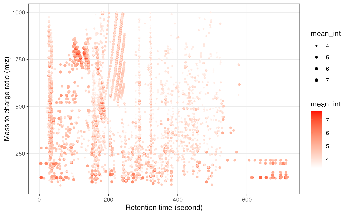
HILIC Negative mode
Load object.
load("mzxml_ms1_data/HILIC/NEG/Result/object")
object_hilic_neg <- object
object_hilic_neg
#> --------------------
#> massdataset version: 0.99.4
#> --------------------
#> 1.expression_data:[ 6557 x 299 data.frame]
#> 2.sample_info:[ 299 x 4 data.frame]
#> 3.variable_info:[ 6557 x 3 data.frame]
#> 4.sample_info_note:[ 4 x 2 data.frame]
#> 5.variable_info_note:[ 3 x 2 data.frame]
#> 6.ms2_data:[ 0 variables x 0 MS2 spectra]
#> --------------------
#> Processing information (extract_process_info())
#> create_mass_dataset ----------
#> Package Function.used Time
#> 1 massdataset create_mass_dataset() 2022-02-28 14:07:06
#> process_data ----------
#> Package Function.used Time
#> 1 massprocesser process_data 2022-02-28 13:05:44Read sample information.
sample_info_neg <- readr::read_csv("sample_info/HILIC/sample_info_neg_1.csv")
#> Rows: 299 Columns: 6
#> ── Column specification ────────────────────────────────────────────────────────
#> Delimiter: ","
#> chr (4): sample_id, class, subject_id, group
#> dbl (2): injection.order, batch
#>
#> ℹ Use `spec()` to retrieve the full column specification for this data.
#> ℹ Specify the column types or set `show_col_types = FALSE` to quiet this message.
head(sample_info_neg)
#> # A tibble: 6 × 6
#> sample_id injection.order class batch subject_id group
#> <chr> <dbl> <chr> <dbl> <chr> <chr>
#> 1 men_normal_166 21 control 1 men_normal_166 male control
#> 2 men_normal_2332 220 control 1 men_normal_2332 male control
#> 3 men_normal_2357 222 control 1 men_normal_2357 male control
#> 4 men_normal_2371 223 control 1 men_normal_2371 male control
#> 5 men_normal_2407 224 control 1 men_normal_2407 male control
#> 6 men_normal_2409 226 control 1 men_normal_2409 male controlAdd sample_info_neg to object_hilic_neg
object_hilic_neg <-
object_hilic_neg %>%
activate_mass_dataset(what = "sample_info") %>%
dplyr::select(-c("group", "class", "injection.order"))
object_hilic_neg <-
object_hilic_neg %>%
activate_mass_dataset(what = "sample_info") %>%
left_join(sample_info_neg,
by = "sample_id")Next, we can get the peak distributation plot of negative mode.
object_hilic_neg %>%
`+`(1) %>%
log(10) %>%
show_mz_rt_plot() +
scale_size_continuous(range = c(0.01, 2))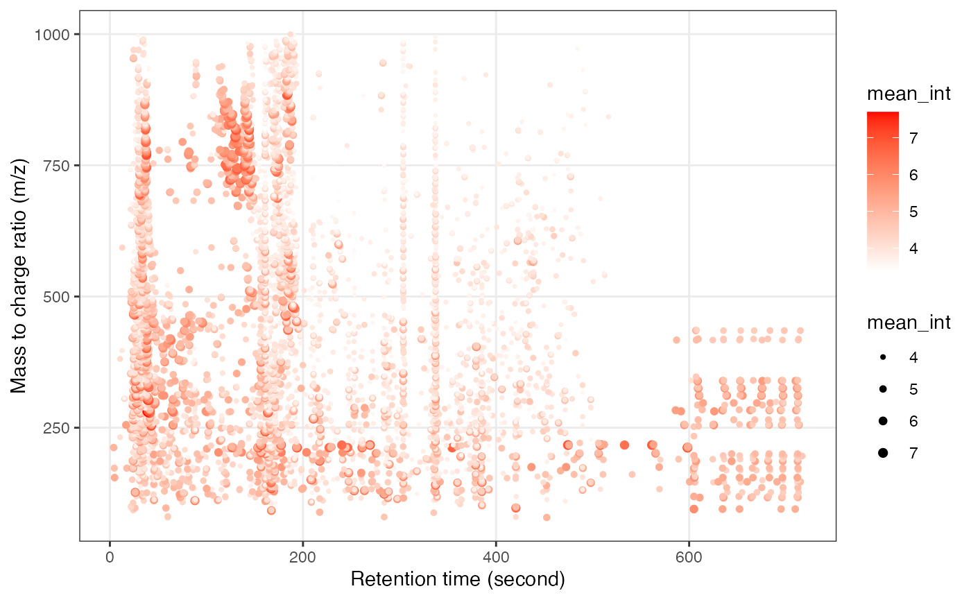
Data cleaning
Data quality assessment before data cleaning
Change batch to character.
object_rplc_pos <-
object_rplc_pos %>%
activate_mass_dataset(what = "sample_info") %>%
dplyr::mutate(batch = as.character(batch))
object_rplc_neg <-
object_rplc_neg %>%
activate_mass_dataset(what = "sample_info") %>%
dplyr::mutate(batch = as.character(batch))
object_hilic_pos <-
object_hilic_pos %>%
activate_mass_dataset(what = "sample_info") %>%
dplyr::mutate(batch = as.character(batch))
object_hilic_neg <-
object_hilic_neg %>%
activate_mass_dataset(what = "sample_info") %>%
dplyr::mutate(batch = as.character(batch))Save them for subsequent analysis.
save(object_rplc_pos, file = "data_cleaning/RPLC/POS/object_rplc_pos")
save(object_rplc_neg, file = "data_cleaning/RPLC/NEG/object_rplc_neg")
save(object_hilic_pos, file = "data_cleaning/HILIC/POS/object_hilic_pos")
save(object_hilic_neg, file = "data_cleaning/HILIC/NEG/object_hilic_neg")Here, we can use the massqc package to assess the data quality.
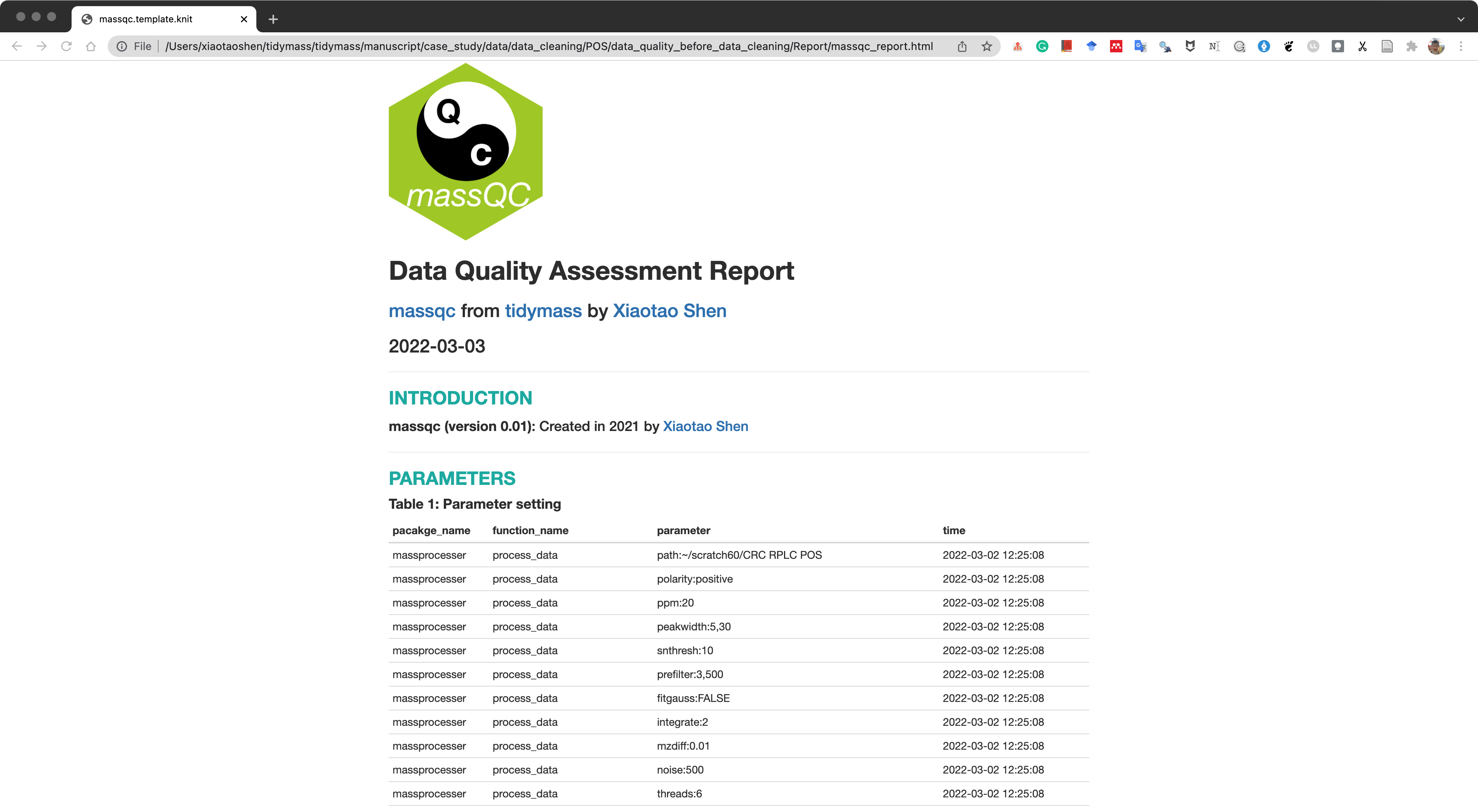
We can just use the massqc_report() function to get a html format quality assessment report.
RPLC Positive mode
massqc::massqc_report(object = object_rplc_pos,
path = "data_cleaning/RPLC/POS/data_quality_before_data_cleaning")A html format report and pdf figures will be placed in the folder data/data_cleaning/POS/data_quality_before_data_cleaning/Report.
The html report is below:
RPLC negative mode.
massqc::massqc_report(object = object_rplc_neg,
path = "data_cleaning/RPLC/NEG/data_quality_before_data_cleaning")HILIC positive mode
massqc::massqc_report(object = object_hilic_pos,
path = "data_cleaning/HILIC/POS/data_quality_before_data_cleaning")HILIC negative mode
massqc::massqc_report(object = object_hilic_neg,
path = "data_cleaning/HILIC/NEG/data_quality_before_data_cleaning")Remove noisy metabolic features
Remove variables which have MVs in more than 20% QC samples and in at lest 50% samples in control group or case group.
RPLC positive mode
object_rplc_pos %>%
activate_mass_dataset(what = "sample_info") %>%
dplyr::count(group)
#> group n
#> 1 female control 14
#> 2 female LCC 50
#> 3 female RCC 60
#> 4 male control 28
#> 5 male LCC 63
#> 6 male RCC 55
#> 7 QC 28MV percentage in QC samples.
show_variable_missing_values(object = object_rplc_pos %>%
activate_mass_dataset(what = "sample_info") %>%
filter(class == "QC"),
percentage = TRUE) +
scale_size_continuous(range = c(0.01, 2))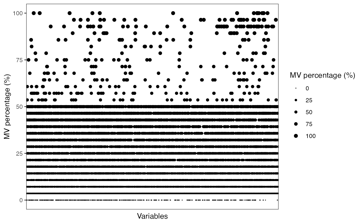
qc_id <-
object_rplc_pos %>%
activate_mass_dataset(what = "sample_info") %>%
filter(class == "QC") %>%
pull(sample_id)
control_id <-
object_rplc_pos %>%
activate_mass_dataset(what = "sample_info") %>%
filter(stringr::str_detect(group, "control")) %>%
pull(sample_id)
case_id <-
object_rplc_pos %>%
activate_mass_dataset(what = "sample_info") %>%
filter(stringr::str_detect(group, "LCC|RCC")) %>%
pull(sample_id)
object_rplc_pos <-
object_rplc_pos %>%
mutate_variable_na_freq(according_to_samples = qc_id) %>%
mutate_variable_na_freq(according_to_samples = control_id) %>%
mutate_variable_na_freq(according_to_samples = case_id)
head(extract_variable_info(object_rplc_pos))
#> variable_id mz rt na_freq na_freq.1 na_freq.2
#> 1 M77T115_POS 77.03846 114.81734 0.1428571 0.2380952 0.1447368
#> 2 M82T641_POS 81.52176 640.56274 0.6071429 0.4523810 0.4956140
#> 3 M82T18_POS 82.01393 18.05400 0.2857143 0.3571429 0.3508772
#> 4 M84T22_POS 84.04433 22.45600 0.3571429 0.3809524 0.3947368
#> 5 M84T19_POS 84.07998 18.99812 0.5000000 0.6666667 0.5131579
#> 6 M85T92_POS 84.96034 92.38353 0.1071429 0.3809524 0.2236842Remove variables.
object_rplc_pos <-
object_rplc_pos %>%
activate_mass_dataset(what = "variable_info") %>%
filter(na_freq < 0.2 &
(na_freq.1 < 0.5 |
na_freq.2 < 0.5))
object_rplc_pos
#> --------------------
#> massdataset version: 0.99.9
#> --------------------
#> 1.expression_data:[ 6132 x 298 data.frame]
#> 2.sample_info:[ 298 x 6 data.frame]
#> 3.variable_info:[ 6132 x 6 data.frame]
#> 4.sample_info_note:[ 6 x 2 data.frame]
#> 5.variable_info_note:[ 6 x 2 data.frame]
#> 6.ms2_data:[ 0 variables x 0 MS2 spectra]
#> --------------------
#> Processing information (extract_process_info())
#> create_mass_dataset ----------
#> Package Function.used Time
#> 1 massdataset create_mass_dataset() 2022-03-02 14:50:02
#> process_data ----------
#> Package Function.used Time
#> 1 massprocesser process_data 2022-03-02 12:25:08
#> mutate ----------
#> Package Function.used Time
#> 1 massdataset mutate() 2022-03-08 22:17:22
#> mutate_variable_na_freq ----------
#> Package Function.used Time
#> 1 massdataset mutate_variable_na_freq() 2022-03-08 22:17:27
#> 2 massdataset mutate_variable_na_freq() 2022-03-08 22:17:27
#> 3 massdataset mutate_variable_na_freq() 2022-03-08 22:17:27
#> filter ----------
#> Package Function.used Time
#> 1 massdataset filter() 2022-03-08 22:17:28Only 6,132 variables left.
RPLC negative mode
qc_id <-
object_rplc_neg %>%
activate_mass_dataset(what = "sample_info") %>%
filter(class == "QC") %>%
pull(sample_id)
control_id <-
object_rplc_neg %>%
activate_mass_dataset(what = "sample_info") %>%
filter(stringr::str_detect(group, "control")) %>%
pull(sample_id)
case_id <-
object_rplc_neg %>%
activate_mass_dataset(what = "sample_info") %>%
filter(stringr::str_detect(group, "LCC|RCC")) %>%
pull(sample_id)
object_rplc_neg =
object_rplc_neg %>%
mutate_variable_na_freq(according_to_samples = qc_id) %>%
mutate_variable_na_freq(according_to_samples = control_id) %>%
mutate_variable_na_freq(according_to_samples = case_id)Remove variables.
object_rplc_neg <-
object_rplc_neg %>%
activate_mass_dataset(what = "variable_info") %>%
filter(
na_freq < 0.2 &
(
na_freq.1 < 0.5 |
na_freq.2 < 0.5
)
)
object_rplc_neg
#> --------------------
#> massdataset version: 0.99.2
#> --------------------
#> 1.expression_data:[ 2719 x 299 data.frame]
#> 2.sample_info:[ 299 x 6 data.frame]
#> 3.variable_info:[ 2719 x 6 data.frame]
#> 4.sample_info_note:[ 6 x 2 data.frame]
#> 5.variable_info_note:[ 6 x 2 data.frame]
#> 6.ms2_data:[ 0 variables x 0 MS2 spectra]
#> --------------------
#> Processing information (extract_process_info())
#> create_mass_dataset ----------
#> Package Function.used Time
#> 1 massdataset create_mass_dataset() 2022-03-01 09:51:34
#> process_data ----------
#> Package Function.used Time
#> 1 massprocesser process_data 2022-03-01 09:03:10
#> mutate ----------
#> Package Function.used Time
#> 1 massdataset mutate() 2022-03-08 22:17:22
#> mutate_variable_na_freq ----------
#> Package Function.used Time
#> 1 massdataset mutate_variable_na_freq() 2022-03-08 22:17:29
#> 2 massdataset mutate_variable_na_freq() 2022-03-08 22:17:29
#> 3 massdataset mutate_variable_na_freq() 2022-03-08 22:17:29
#> filter ----------
#> Package Function.used Time
#> 1 massdataset filter() 2022-03-08 22:17:292,719 features left.
HILIC positive mode
qc_id <-
object_hilic_pos %>%
activate_mass_dataset(what = "sample_info") %>%
filter(class == "QC") %>%
pull(sample_id)
control_id <-
object_hilic_pos %>%
activate_mass_dataset(what = "sample_info") %>%
filter(stringr::str_detect(group, "control")) %>%
pull(sample_id)
case_id <-
object_hilic_pos %>%
activate_mass_dataset(what = "sample_info") %>%
filter(stringr::str_detect(group, "LCC|RCC")) %>%
pull(sample_id)
object_hilic_pos =
object_hilic_pos %>%
mutate_variable_na_freq(according_to_samples = qc_id) %>%
mutate_variable_na_freq(according_to_samples = control_id) %>%
mutate_variable_na_freq(according_to_samples = case_id)Remove variables.
object_hilic_pos <-
object_hilic_pos %>%
activate_mass_dataset(what = "variable_info") %>%
filter(
na_freq < 0.2 &
(
na_freq.1 < 0.5 |
na_freq.2 < 0.5
)
)
object_rplc_neg
#> --------------------
#> massdataset version: 0.99.2
#> --------------------
#> 1.expression_data:[ 2719 x 299 data.frame]
#> 2.sample_info:[ 299 x 6 data.frame]
#> 3.variable_info:[ 2719 x 6 data.frame]
#> 4.sample_info_note:[ 6 x 2 data.frame]
#> 5.variable_info_note:[ 6 x 2 data.frame]
#> 6.ms2_data:[ 0 variables x 0 MS2 spectra]
#> --------------------
#> Processing information (extract_process_info())
#> create_mass_dataset ----------
#> Package Function.used Time
#> 1 massdataset create_mass_dataset() 2022-03-01 09:51:34
#> process_data ----------
#> Package Function.used Time
#> 1 massprocesser process_data 2022-03-01 09:03:10
#> mutate ----------
#> Package Function.used Time
#> 1 massdataset mutate() 2022-03-08 22:17:22
#> mutate_variable_na_freq ----------
#> Package Function.used Time
#> 1 massdataset mutate_variable_na_freq() 2022-03-08 22:17:29
#> 2 massdataset mutate_variable_na_freq() 2022-03-08 22:17:29
#> 3 massdataset mutate_variable_na_freq() 2022-03-08 22:17:29
#> filter ----------
#> Package Function.used Time
#> 1 massdataset filter() 2022-03-08 22:17:29HILIC negative mode
qc_id <-
object_hilic_neg %>%
activate_mass_dataset(what = "sample_info") %>%
filter(class == "QC") %>%
pull(sample_id)
control_id <-
object_hilic_neg %>%
activate_mass_dataset(what = "sample_info") %>%
filter(stringr::str_detect(group, "control")) %>%
pull(sample_id)
case_id <-
object_hilic_neg %>%
activate_mass_dataset(what = "sample_info") %>%
filter(stringr::str_detect(group, "LCC|RCC")) %>%
pull(sample_id)
object_hilic_neg =
object_hilic_neg %>%
mutate_variable_na_freq(according_to_samples = qc_id) %>%
mutate_variable_na_freq(according_to_samples = control_id) %>%
mutate_variable_na_freq(according_to_samples = case_id)Remove variables.
object_hilic_neg <-
object_hilic_neg %>%
activate_mass_dataset(what = "variable_info") %>%
filter(
na_freq < 0.2 &
(
na_freq.1 < 0.5 |
na_freq.2 < 0.5
)
)
object_hilic_neg
#> --------------------
#> massdataset version: 0.99.4
#> --------------------
#> 1.expression_data:[ 3808 x 299 data.frame]
#> 2.sample_info:[ 299 x 6 data.frame]
#> 3.variable_info:[ 3808 x 6 data.frame]
#> 4.sample_info_note:[ 6 x 2 data.frame]
#> 5.variable_info_note:[ 6 x 2 data.frame]
#> 6.ms2_data:[ 0 variables x 0 MS2 spectra]
#> --------------------
#> Processing information (extract_process_info())
#> create_mass_dataset ----------
#> Package Function.used Time
#> 1 massdataset create_mass_dataset() 2022-02-28 14:07:06
#> process_data ----------
#> Package Function.used Time
#> 1 massprocesser process_data 2022-02-28 13:05:44
#> mutate ----------
#> Package Function.used Time
#> 1 massdataset mutate() 2022-03-08 22:17:22
#> mutate_variable_na_freq ----------
#> Package Function.used Time
#> 1 massdataset mutate_variable_na_freq() 2022-03-08 22:17:31
#> 2 massdataset mutate_variable_na_freq() 2022-03-08 22:17:31
#> 3 massdataset mutate_variable_na_freq() 2022-03-08 22:17:31
#> filter ----------
#> Package Function.used Time
#> 1 massdataset filter() 2022-03-08 22:17:32Filter outlier samples
We can use the detect_outlier() to find the outlier samples.
More information about how to detect outlier samples can be found here.
RPLC positive mode
##change class to subject
object_rplc_pos <-
object_rplc_pos %>%
activate_mass_dataset(what = "sample_info") %>%
dplyr::mutate(class = case_when(class == "QC" ~ class,
TRUE ~ "Subject"))Detect outlier samples.
outlier_samples <-
object_rplc_pos %>%
`+`(1) %>%
log(2) %>%
scale() %>%
detect_outlier(na_percentage_cutoff = 0.5)
outlier_samples
#> --------------------
#> masscleaner
#> --------------------
#> 1 according_to_na : 11 outlier samples.
#> menLCCstage1_2516,menLCCstage2_134,menRCCstage2_2498,menRCCstage2_2520,women_normal_2478,... .
#> 2 according_to_pc_sd : 0 outlier samples.
#> 3 according_to_pc_mad : 0 outlier samples.
#> 4 accordint_to_distance : 0 outlier samples.
#> extract all outlier table using extract_outlier_table()
#>
outlier_table <-
extract_outlier_table(outlier_samples)
outlier_table %>%
apply(1, function(x){
sum(x)
}) %>%
`>`(0) %>%
which()
#> menLCCstage1_2516 menLCCstage2_134 menRCCstage2_2498 menRCCstage2_2520
#> 34 48 117 118
#> women_normal_2478 women_normal_2495 womenLCCstage1_577 womenRCCstage2_1733
#> 149 150 170 236
#> womenRCCstage3_2249 womenRCCstage3_2494 QC28
#> 263 265 298Here, we don’t remove outlier samples.
RPLC negative mode
##change class to subject
object_rplc_neg <-
object_rplc_neg %>%
activate_mass_dataset(what = "sample_info") %>%
dplyr::mutate(class = case_when(class == "QC" ~ class,
TRUE ~ "Subject"))Detect outlier samples.
outlier_samples <-
object_rplc_neg %>%
`+`(1) %>%
log(2) %>%
scale() %>%
detect_outlier()
outlier_samples
#> --------------------
#> masscleaner
#> --------------------
#> 1 according_to_na : 8 outlier samples.
#> men_normal_363,menLCCstage2_134,menLCCstage2_714,women_normal_11,womenLCCstage1_577,... .
#> 2 according_to_pc_sd : 0 outlier samples.
#> 3 according_to_pc_mad : 0 outlier samples.
#> 4 accordint_to_distance : 0 outlier samples.
#> extract all outlier table using extract_outlier_table()
#> HILIC positive mode
##change class to subject
object_hilic_pos <-
object_hilic_pos %>%
activate_mass_dataset(what = "sample_info") %>%
dplyr::mutate(class = case_when(class == "QC" ~ class,
TRUE ~ "Subject"))Detect outlier samples.
outlier_samples <-
object_hilic_pos %>%
`+`(1) %>%
log(2) %>%
scale() %>%
detect_outlier()
outlier_samples
#> --------------------
#> masscleaner
#> --------------------
#> 1 according_to_na : 6 outlier samples.
#> men_normal_2518,menLCCstage1_2516,menRCCstage2_2498,menRCCstage2_2520,women_normal_2495,... .
#> 2 according_to_pc_sd : 0 outlier samples.
#> 3 according_to_pc_mad : 0 outlier samples.
#> 4 accordint_to_distance : 0 outlier samples.
#> extract all outlier table using extract_outlier_table()
#> HILIC negative mode
##change class to subject
object_hilic_neg <-
object_hilic_neg %>%
activate_mass_dataset(what = "sample_info") %>%
dplyr::mutate(class = case_when(class == "QC" ~ class,
TRUE ~ "Subject"))Detect outlier samples.
outlier_samples <-
object_hilic_neg %>%
`+`(1) %>%
log(2) %>%
scale() %>%
detect_outlier()
outlier_samples
#> --------------------
#> masscleaner
#> --------------------
#> 1 according_to_na : 2 outlier samples.
#> menRCCstage2_2520,womenRCCstage3_2494 .
#> 2 according_to_pc_sd : 0 outlier samples.
#> 3 according_to_pc_mad : 0 outlier samples.
#> 4 accordint_to_distance : 0 outlier samples.
#> extract all outlier table using extract_outlier_table()
#> Missing value imputation
object_rplc_pos <-
impute_mv(object = object_rplc_pos,
method = "knn", colmax = 0.9)
object_rplc_neg <-
impute_mv(object = object_rplc_neg, method = "knn")
object_hilic_pos <-
impute_mv(object = object_hilic_pos, method = "knn")
object_hilic_neg <-
impute_mv(object = object_hilic_neg, method = "knn")Data normalization and integration
RPLC positive mode
load("data_cleaning/RPLC/POS/object_rplc_pos")
object_rplc_pos <-
normalize_data(object_rplc_pos, method = "svr")
object_rplc_pos2 <-
integrate_data(object_rplc_pos, method = "subject_median")Save it for subsequent analysis.
save(object_rplc_pos2, file = "data_cleaning/RPLC/POS/object_rplc_pos2")RPLC negative mode
load("data_cleaning/RPLC/NEG/object_rplc_neg")
object_rplc_neg <-
normalize_data(object_rplc_neg, method = "svr")
object_rplc_neg2 <-
integrate_data(object_rplc_neg, method = "subject_median")Save it for subsequent analysis.
save(object_rplc_neg2, file = "data_cleaning/RPLC/NEG/object_rplc_neg2")HILIC positive mode
load("data_cleaning/HILIC/POS/object_hilic_pos")
object_hilic_pos <-
normalize_data(object_hilic_pos, method = "svr")
object_hilic_pos2 <-
integrate_data(object_hilic_pos, method = "subject_median")Save it for subsequent analysis.
save(object_hilic_pos2, file = "data_cleaning/HILIC/POS/object_hilic_pos2")HILIC negative mode
load("data_cleaning/HILIC/NEG/object_hilic_neg")
object_hilic_neg <-
normalize_data(object_hilic_neg, method = "svr")
object_hilic_neg2 <-
integrate_data(object_hilic_neg, method = "subject_median")Save it for subsequent analysis.
save(object_hilic_neg2, file = "data_cleaning/HILIC/NEG/object_hilic_neg2")Data quality assessment after data cleaning
We can use the massqc_report() function to get a html format quality assessment report.
load("data_cleaning/RPLC/POS/object_rplc_pos2")
massqc::massqc_report(object = object_rplc_pos2,
path = "data_cleaning/RPLC/POS/data_quality_after_data_cleaning")
load("data_cleaning/RPLC/NEG/object_rplc_neg2")
massqc::massqc_report(object = object_rplc_neg2,
path = "data_cleaning/RPLC/NEG/data_quality_after_data_cleaning")
load("data_cleaning/HILIC/POS/object_hilic_pos2")
massqc::massqc_report(object = object_hilic_pos2,
path = "data_cleaning/HILIC/POS/data_quality_after_data_cleaning")
load("data_cleaning/HILIC/NEG/object_hilic_neg2")
massqc::massqc_report(object = object_hilic_neg2,
path = "data_cleaning/HILIC/NEG/data_quality_after_data_cleaning")Metabolite annotation
Add MS2 spectra to object
Download the MS2 data here.
Place it in the data folder and uncompress it.
RPLC positive mode
object_rplc_pos2 <-
mutate_ms2(
object = object_rplc_pos2,
column = "rplc",
polarity = "positive",
ms1.ms2.match.mz.tol = 5,
ms1.ms2.match.rt.tol = 30,
path = "mgf_ms2_data/RPLC/POS/"
)RPLC negative mode
object_rplc_neg2 <-
mutate_ms2(
object = object_rplc_neg2,
column = "rplc",
polarity = "negative",
ms1.ms2.match.mz.tol = 5,
ms1.ms2.match.rt.tol = 30,
path = "mgf_ms2_data/RPLC/NEG/"
)HILIC positive mode
object_hilic_pos2 <-
mutate_ms2(
object = object_hilic_pos2,
column = "hilic",
polarity = "positive",
ms1.ms2.match.mz.tol = 5,
ms1.ms2.match.rt.tol = 30,
path = "mgf_ms2_data/HILIC/POS/"
)Metabolite annotation using metid
Metabolite annotation is based on the metid package.
Download database
We need to download MS1 and MS2 database from metid website.
The in-house database is constructed with MS1 and RT information.
We also download the public databases, snyder_database_hilic0.0.3. And place them in a new folder named as metabolite_annotation.
RPLC positive mode
Annotate features using in-house database.
load("metabolite_annotation/database/RPLC.database")
object_rplc_pos3 <-
annotate_metabolites_mass_dataset(object = object_rplc_pos2,
ms1.match.ppm = 15,
rt.match.tol = 30,
polarity = "positive",
database = RPLC.database)Annotate features using snyder_database_rplc0.0.3.
load("metabolite_annotation/database/snyder_database_rplc0.0.3")
object_rplc_pos3 <-
annotate_metabolites_mass_dataset(object = object_rplc_pos3,
ms1.match.ppm = 15,
rt.match.tol = 1000000,
polarity = "positive",
database = snyder_database_rplc0.0.3)Save it for subsequent analysis.
save(object_rplc_pos3, file = "metabolite_annotation/RPLC/POS/object_rplc_pos3")RPLC negative mode
Annotate features using in-house database.
object_rplc_neg3 <-
annotate_metabolites_mass_dataset(object = object_rplc_neg2,
ms1.match.ppm = 15,
rt.match.tol = 30,
polarity = "negative",
database = RPLC.database)Annotate features using snyder_database_rplc0.0.3.
object_rplc_neg3 <-
annotate_metabolites_mass_dataset(object = object_rplc_neg3,
ms1.match.ppm = 15,
rt.match.tol = 1000000,
polarity = "negative",
database = snyder_database_rplc0.0.3)Save it for subsequent analysis.
save(object_rplc_neg3, file = "metabolite_annotation/RPLC/NEG/object_rplc_neg3")HILIC positive mode
Annotate features using in-house database.
load("metabolite_annotation/database/HILIC.database")
object_hilic_pos3 <-
annotate_metabolites_mass_dataset(object = object_hilic_pos2,
ms1.match.ppm = 15,
rt.match.tol = 30,
polarity = "positive",
database = HILIC.database)Annotate features using snyder_database_hilic0.0.3.
load("metabolite_annotation/database/snyder_database_hilic0.0.3")
object_hilic_pos3 <-
annotate_metabolites_mass_dataset(object = object_hilic_pos3,
ms1.match.ppm = 15,
rt.match.tol = 1000000,
polarity = "positive",
database = snyder_database_hilic0.0.3)Save it for subsequent analysis.
save(object_hilic_pos3, file = "metabolite_annotation/HILIC/POS/object_hilic_pos3")HILIC negative mode
Annotate features using in-house database.
object_hilic_neg3 <-
annotate_metabolites_mass_dataset(object = object_hilic_neg2,
ms1.match.ppm = 15,
rt.match.tol = 30,
polarity = "negative",
database = HILIC.database)Annotate features using snyder_database_hilic0.0.3.
object_hilic_neg3 <-
annotate_metabolites_mass_dataset(object = object_hilic_neg3,
ms1.match.ppm = 15,
rt.match.tol = 1000000,
polarity = "negative",
database = snyder_database_hilic0.0.3)Save it for subsequent analysis.
save(object_hilic_neg3, file = "metabolite_annotation/HILIC/NEG/object_hilic_neg3")Annotation result
load("metabolite_annotation/RPLC/POS/object_rplc_pos3")
load("metabolite_annotation/RPLC/NEG/object_rplc_neg3")
load("metabolite_annotation/HILIC/POS/object_hilic_pos3")
load("metabolite_annotation/HILIC/NEG/object_hilic_neg3")The annotation result can be got using the extract_annotation_table function.
head(extract_annotation_table(object = object_rplc_pos3))
#> variable_id ms2_files_id ms2_spectrum_id
#> 1 M1000T389_POS NA NA
#> 2 M1000T389_POS NA NA
#> 3 M103T115_1_POS NA NA
#> 4 M105T218_POS NA NA
#> 5 M105T218_POS NA NA
#> 6 M105T22_POS NA NA
#> Compound.name CAS.ID HMDB.ID KEGG.ID Lab.ID
#> 1 Tauroursodeoxycholic acid 14605-22-2 HMDB00874 <NA> RPLC_882
#> 2 Tauroursodeoxycholic acid 14605-22-2 HMDB00874 <NA> RPLC_643
#> 3 2-(4-Hydroxyphenyl)ethanol (Tyrosol) <NA> <NA> <NA> RPLC_9
#> 4 BENZOATE <NA> <NA> <NA> RPLC_329
#> 5 4-HYDROXYBENZALDEHYDE <NA> <NA> <NA> RPLC_365
#> 6 N,N-Dimethylguanidine sulfate <NA> <NA> <NA> RPLC_41
#> Adduct mz.error mz.match.score RT.error RT.match.score CE SS
#> 1 (2M+H)+ 6.990604 0.8970921 NA NA NA NA
#> 2 (2M+H)+ 8.591256 0.8487238 NA NA NA NA
#> 3 (M+H-2H2O)+ 1.199677 0.9968068 NA NA NA NA
#> 4 (M+H-H2O)+ 1.322858 0.9961188 NA NA NA NA
#> 5 (M+H-H2O)+ 1.322858 0.9961188 NA NA NA NA
#> 6 (M+NH4)+ 10.611103 0.7786355 NA NA NA NA
#> Total.score Database Level
#> 1 0.8970921 MS_0.0.2 3
#> 2 0.8487238 MS_0.0.2 3
#> 3 0.9968068 MS_0.0.2 3
#> 4 0.9961188 MS_0.0.2 3
#> 5 0.9961188 MS_0.0.2 3
#> 6 0.7786355 MS_0.0.2 3
variable_info_pos <-
extract_variable_info(object = object_rplc_pos3)
head(variable_info_pos)
#> variable_id mz rt na_freq na_freq.1 na_freq.2
#> 1 M77T115_POS 77.03846 114.81734 0.14285714 0.2380952 0.14473684
#> 2 M85T92_POS 84.96034 92.38353 0.10714286 0.3809524 0.22368421
#> 3 M90T23_POS 90.05328 23.39891 0.03571429 0.2619048 0.17982456
#> 4 M91T52_POS 91.05412 51.77000 0.10714286 0.1904762 0.10526316
#> 5 M91T115_POS 91.05412 114.80016 0.03571429 0.2142857 0.16228070
#> 6 M95T115_POS 95.04891 114.80017 0.10714286 0.1190476 0.09210526
#> Compound.name CAS.ID HMDB.ID KEGG.ID Lab.ID Adduct
#> 1 PHENOL <NA> <NA> <NA> RPLC_308 (M+H-H2O)+
#> 2 <NA> <NA> <NA> <NA> <NA> <NA>
#> 3 BETA-ALANINE <NA> <NA> <NA> RPLC_288 (M+H)+
#> 4 <NA> <NA> <NA> <NA> <NA> <NA>
#> 5 <NA> <NA> <NA> <NA> <NA> <NA>
#> 6 4-METHYL-2-OXO-PENTANOIC ACID <NA> <NA> <NA> RPLC_291 (M+H-2H2O)+
#> mz.error mz.match.score RT.error RT.match.score CE SS Total.score Database
#> 1 0.2755554 0.9998313 NA NA NA NA 0.9998313 MS_0.0.2
#> 2 NA NA NA NA NA NA NA <NA>
#> 3 4.2407715 0.9608233 NA NA NA NA 0.9608233 MS_0.0.2
#> 4 NA NA NA NA NA NA NA <NA>
#> 5 NA NA NA NA NA NA NA <NA>
#> 6 0.4448792 0.9995603 NA NA NA NA 0.9995603 MS_0.0.2
#> Level
#> 1 3
#> 2 NA
#> 3 3
#> 4 NA
#> 5 NA
#> 6 3Statistical analysis and pathway analysis
Remove the features without annotations
We only remain the annotations with level 2.
Merge data
We need to merge RPLC, HILIC positive and negative mode data as one mass_dataset class.
head(colnames(object_rplc_pos3))
#> [1] "men_normal_166" "men_normal_2332" "men_normal_2357" "men_normal_2371"
#> [5] "men_normal_2407" "men_normal_2409"
head(colnames(object_rplc_neg3))
#> [1] "men_normal_166" "men_normal_2332" "men_normal_2357" "men_normal_2371"
#> [5] "men_normal_2407" "men_normal_2409"
head(colnames(object_hilic_pos3))
#> [1] "men_normal_166" "men_normal_2332" "men_normal_2357" "men_normal_2371"
#> [5] "men_normal_2407" "men_normal_2409"
head(colnames(object_hilic_neg3))
#> [1] "menLCCstage1_1122" "menLCCstage1_1487" "menLCCstage1_1532"
#> [4] "menLCCstage1_1941" "menLCCstage1_1969" "menLCCstage1_2516"
object_rplc <-
merge_mass_dataset(
x = object_rplc_pos3,
y = object_rplc_neg3,
sample_direction = "inner",
variable_direction = "full",
sample_by = "sample_id",
variable_by = c("variable_id", "mz", "rt")
)
object_hilic <-
merge_mass_dataset(
x = object_hilic_pos3,
y = object_hilic_neg3,
sample_direction = "inner",
variable_direction = "full",
sample_by = "sample_id",
variable_by = c("variable_id", "mz", "rt")
)
object <-
merge_mass_dataset(
x = object_rplc,
y = object_hilic,
sample_direction = "inner",
variable_direction = "full",
sample_by = "sample_id",
variable_by = c("variable_id", "mz", "rt")
)
object
#> --------------------
#> massdataset version: 0.99.20
#> --------------------
#> 1.expression_data:[ 169 x 298 data.frame]
#> 2.sample_info:[ 298 x 21 data.frame]
#> 3.variable_info:[ 169 x 15 data.frame]
#> 4.sample_info_note:[ 21 x 2 data.frame]
#> 5.variable_info_note:[ 15 x 2 data.frame]
#> 6.ms2_data:[ 0 variables x 0 MS2 spectra]
#> --------------------
#> Processing information (extract_process_info())
#> create_mass_dataset ----------
#> Package Function.used Time
#> 1 massdataset create_mass_dataset() 2022-03-02 14:50:02
#> process_data ----------
#> Package Function.used Time
#> 1 massprocesser process_data 2022-03-02 12:25:08
#> mutate ----------
#> Package Function.used Time
#> 1 massdataset mutate() 2022-03-05 16:52:56
#> 2 massdataset mutate() 2022-03-05 17:08:57
#> mutate_variable_na_freq ----------
#> Package Function.used Time
#> 1 massdataset mutate_variable_na_freq() 2022-03-05 17:01:27
#> 2 massdataset mutate_variable_na_freq() 2022-03-05 17:01:27
#> 3 massdataset mutate_variable_na_freq() 2022-03-05 17:01:27
#> filter ----------
#> Package Function.used Time
#> 1 massdataset filter() 2022-03-05 17:01:37
#> 2 massdataset filter() 2022-03-08 22:18:13
#> 3 massdataset filter() 2022-03-08 22:18:13
#> impute_mv ----------
#> Package Function.used Time
#> 1 masscleaner impute_mv() 2022-03-05 17:45:56
#> normalize_data ----------
#> Package Function.used Time
#> 1 masscleaner normalize_data() 2022-03-05 19:18:27
#> annotate_metabolites_mass_dataset ----------
#> Package Function.used Time
#> 1 metid annotate_metabolites_mass_dataset() 2022-03-05 23:36:53
#> 2 metid annotate_metabolites_mass_dataset() 2022-03-06 00:13:48
#> create_mass_dataset ----------
#> Package Function.used Time
#> 1 massdataset create_mass_dataset() 2022-03-01 09:51:34
#> process_data ----------
#> Package Function.used Time
#> 1 massprocesser process_data 2022-03-01 09:03:10
#> mutate ----------
#> Package Function.used Time
#> 1 massdataset mutate() 2022-03-05 16:53:03
#> 2 massdataset mutate() 2022-03-05 17:10:13
#> mutate_variable_na_freq ----------
#> Package Function.used Time
#> 1 massdataset mutate_variable_na_freq() 2022-03-05 17:04:03
#> 2 massdataset mutate_variable_na_freq() 2022-03-05 17:04:03
#> 3 massdataset mutate_variable_na_freq() 2022-03-05 17:04:03
#> filter ----------
#> Package Function.used Time
#> 1 massdataset filter() 2022-03-05 17:04:15
#> 2 massdataset filter() 2022-03-08 22:18:13
#> 3 massdataset filter() 2022-03-08 22:18:13
#> impute_mv ----------
#> Package Function.used Time
#> 1 masscleaner impute_mv() 2022-03-05 17:46:18
#> normalize_data ----------
#> Package Function.used Time
#> 1 masscleaner normalize_data() 2022-03-05 19:56:37
#> annotate_metabolites_mass_dataset ----------
#> Package Function.used Time
#> 1 metid annotate_metabolites_mass_dataset() 2022-03-06 00:29:13
#> 2 metid annotate_metabolites_mass_dataset() 2022-03-06 00:36:58
#> merge_mass_dataset ----------
#> Package Function.used Time
#> 1 massdataset merge_mass_dataset 2022-03-08 22:18:14
#> 2 massdataset merge_mass_dataset 2022-03-08 22:18:15
#> create_mass_dataset ----------
#> Package Function.used Time
#> 1 massdataset create_mass_dataset() 2022-03-02 09:06:33
#> process_data ----------
#> Package Function.used Time
#> 1 massprocesser process_data 2022-03-02 07:55:29
#> mutate ----------
#> Package Function.used Time
#> 1 massdataset mutate() 2022-03-05 16:53:24
#> 2 massdataset mutate() 2022-03-05 17:18:51
#> mutate_variable_na_freq ----------
#> Package Function.used Time
#> 1 massdataset mutate_variable_na_freq() 2022-03-05 17:06:07
#> 2 massdataset mutate_variable_na_freq() 2022-03-05 17:06:07
#> 3 massdataset mutate_variable_na_freq() 2022-03-05 17:06:08
#> filter ----------
#> Package Function.used Time
#> 1 massdataset filter() 2022-03-05 17:06:16
#> 2 massdataset filter() 2022-03-08 22:18:14
#> 3 massdataset filter() 2022-03-08 22:18:14
#> impute_mv ----------
#> Package Function.used Time
#> 1 masscleaner impute_mv() 2022-03-05 17:46:40
#> normalize_data ----------
#> Package Function.used Time
#> 1 masscleaner normalize_data() 2022-03-05 20:54:20
#> annotate_metabolites_mass_dataset ----------
#> Package Function.used Time
#> 1 metid annotate_metabolites_mass_dataset() 2022-03-06 00:43:12
#> 2 metid annotate_metabolites_mass_dataset() 2022-03-06 00:48:51
#> create_mass_dataset ----------
#> Package Function.used Time
#> 1 massdataset create_mass_dataset() 2022-02-28 14:07:06
#> process_data ----------
#> Package Function.used Time
#> 1 massprocesser process_data 2022-02-28 13:05:44
#> mutate ----------
#> Package Function.used Time
#> 1 massdataset mutate() 2022-03-05 16:53:35
#> 2 massdataset mutate() 2022-03-05 17:19:31
#> mutate_variable_na_freq ----------
#> Package Function.used Time
#> 1 massdataset mutate_variable_na_freq() 2022-03-05 17:08:15
#> 2 massdataset mutate_variable_na_freq() 2022-03-05 17:08:15
#> 3 massdataset mutate_variable_na_freq() 2022-03-05 17:08:15
#> filter ----------
#> Package Function.used Time
#> 1 massdataset filter() 2022-03-05 17:08:20
#> 2 massdataset filter() 2022-03-08 22:18:14
#> 3 massdataset filter() 2022-03-08 22:18:14
#> impute_mv ----------
#> Package Function.used Time
#> 1 masscleaner impute_mv() 2022-03-05 17:46:54
#> normalize_data ----------
#> Package Function.used Time
#> 1 masscleaner normalize_data() 2022-03-05 21:06:01
#> annotate_metabolites_mass_dataset ----------
#> Package Function.used Time
#> 1 metid annotate_metabolites_mass_dataset() 2022-03-06 00:58:51
#> 2 metid annotate_metabolites_mass_dataset() 2022-03-06 01:14:54
#> merge_mass_dataset ----------
#> Package Function.used Time
#> 1 massdataset merge_mass_dataset 2022-03-08 22:18:14Remove redundant metabolites
Remove the redundant annotated metabolites bases on Level and score.
object <-
object %>%
activate_mass_dataset(what = "annotation_table") %>%
group_by(Compound.name) %>%
filter(Level == min(Level)) %>%
filter(Total.score == max(Total.score)) %>%
slice_head(n = 1)Save it for subsequent analysis.
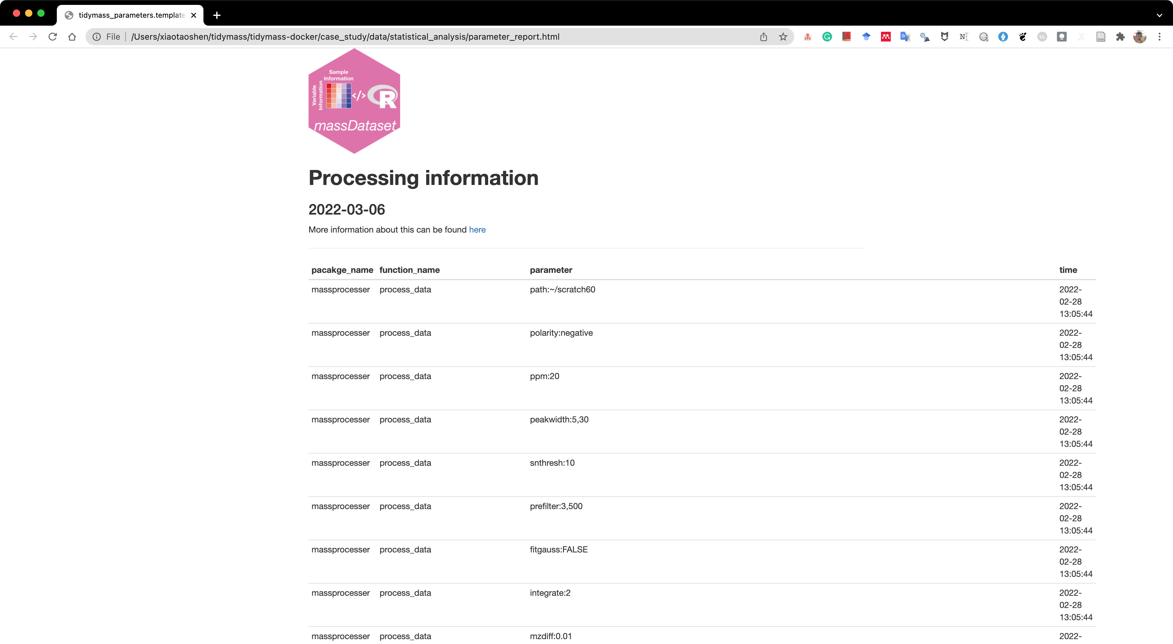
save(object, file = "statistical_analysis/object")Trace processing information of object
Then we can use the report_parameters() function to trace processing information of object.
All the analysis results will be placed in a folder named as statistical_analysis.
report_parameters(object = object, path = "statistical_analysis")A html format file named as parameter_report.html will be generated.
Clustering of all samples
load("statistical_analysis/object")
temp_object <-
object %>%
activate_mass_dataset(what = "sample_info") %>%
filter(group != "QC") %>%
`+`(1) %>%
log(2) %>%
scale()
library(ComplexHeatmap)
h1 <- HeatmapAnnotation(class = extract_sample_info(temp_object)$group)
massstat::Heatmap(matrix = temp_object,
name = "z-score",
row_names_gp = gpar(cex = 0.2),
column_names_gp = gpar(cex = 0.2),
top_annotation = h1)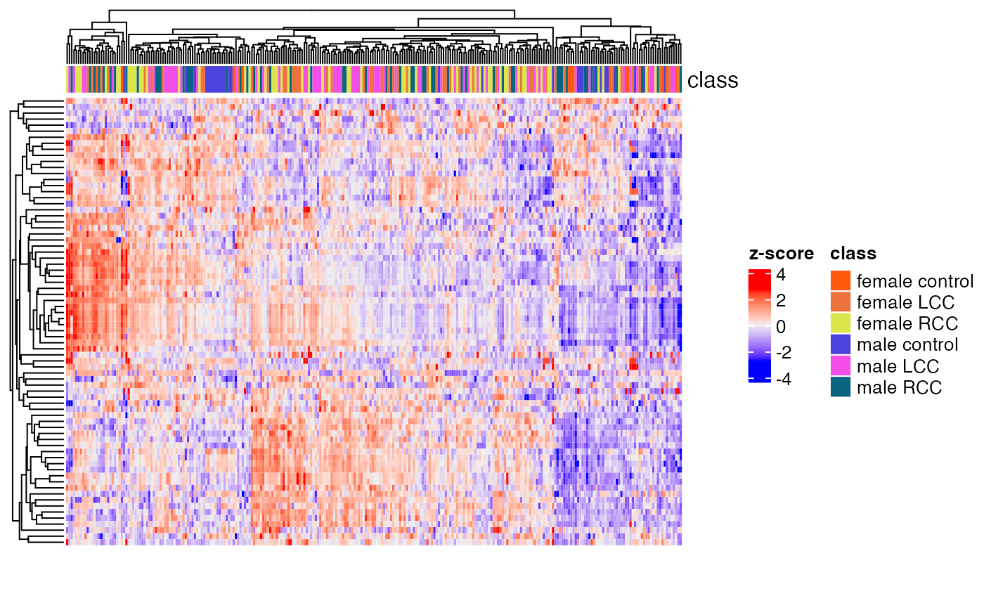
Differential expression metabolites
We want to see if the dysregulated metabolites and pathways are different in males and female cancer tissues.
Calculate the fold changes.
femaleLCC <-
object %>%
activate_mass_dataset(what = "sample_info") %>%
dplyr::filter(group == "female LCC") %>%
dplyr::pull(sample_id)
femaleRCC <-
object %>%
activate_mass_dataset(what = "sample_info") %>%
dplyr::filter(group == "female RCC") %>%
dplyr::pull(sample_id)
maleLCC <-
object %>%
activate_mass_dataset(what = "sample_info") %>%
dplyr::filter(group == "male LCC") %>%
dplyr::pull(sample_id)
maleRCC <-
object %>%
activate_mass_dataset(what = "sample_info") %>%
dplyr::filter(group == "male RCC") %>%
dplyr::pull(sample_id)
femalecontrol <-
object %>%
activate_mass_dataset(what = "sample_info") %>%
dplyr::filter(group == "female control") %>%
dplyr::pull(sample_id)
malecontrol <-
object %>%
activate_mass_dataset(what = "sample_info") %>%
dplyr::filter(group == "male control") %>%
dplyr::pull(sample_id)Calculate p values
object <-
mutate_p_value(
object = object,
control_sample_id = malecontrol,
case_sample_id = maleLCC,
method = "t.test",
p_adjust_methods = "BH"
)
#> 28 control samples.
#> 63 case samples.
#>
object <-
object %>%
activate_mass_dataset(what = "variable_info") %>%
dplyr::rename(p_value_malelcc_vs_malecontrol = p_value,
p_value_adjust_malelcc_vs_malecontrol = p_value_adjust)
object <-
mutate_p_value(
object = object,
control_sample_id = femalecontrol,
case_sample_id = femaleLCC,
method = "t.test",
p_adjust_methods = "BH"
)
#> 14 control samples.
#> 50 case samples.
#>
object <-
object %>%
activate_mass_dataset(what = "variable_info") %>%
dplyr::rename(p_value_femalelcc_vs_femalecontrol = p_value,
p_value_adjust_femalelcc_vs_femalecontrol = p_value_adjust)Volcano plot
plot <-
volcano_plot(object = object,
fc_column_name = "fc_femalelcc_vs_femalecontrol",
p_value_column_name = "p_value_adjust_femalelcc_vs_femalecontrol",
add_text = TRUE,
text_from = "Compound.name",
fc_up_cutoff = 1,
fc_down_cutoff = 1,
p_value_cutoff = 0.05,
point_size_scale = "p_value_adjust_femalelcc_vs_femalecontrol") +
scale_size_continuous(range = c(0.5, 5))
plot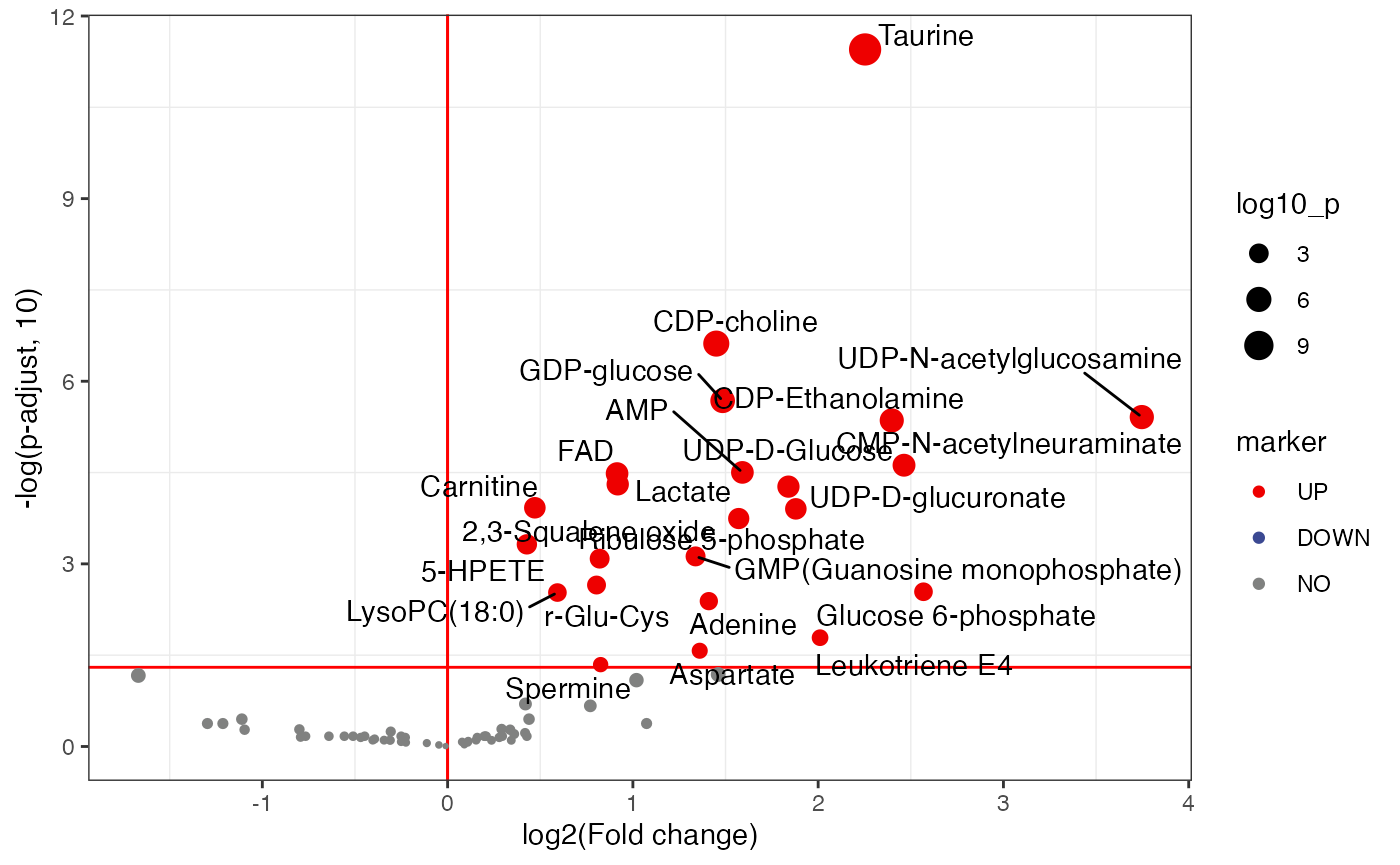
ggsave(plot, filename = "statistical_analysis/female_LCC_vs_femal_control.pdf", width = 8, height = 7)
plot <-
volcano_plot(object = object,
fc_column_name = "fc_malelcc_vs_malecontrol",
p_value_column_name = "p_value_adjust_malelcc_vs_malecontrol",
add_text = TRUE,
text_from = "Compound.name",
fc_up_cutoff = 1,
fc_down_cutoff = 1,
p_value_cutoff = 0.05,
point_size_scale = "p_value_adjust_malelcc_vs_malecontrol") +
scale_size_continuous(range = c(0.5, 5))
plot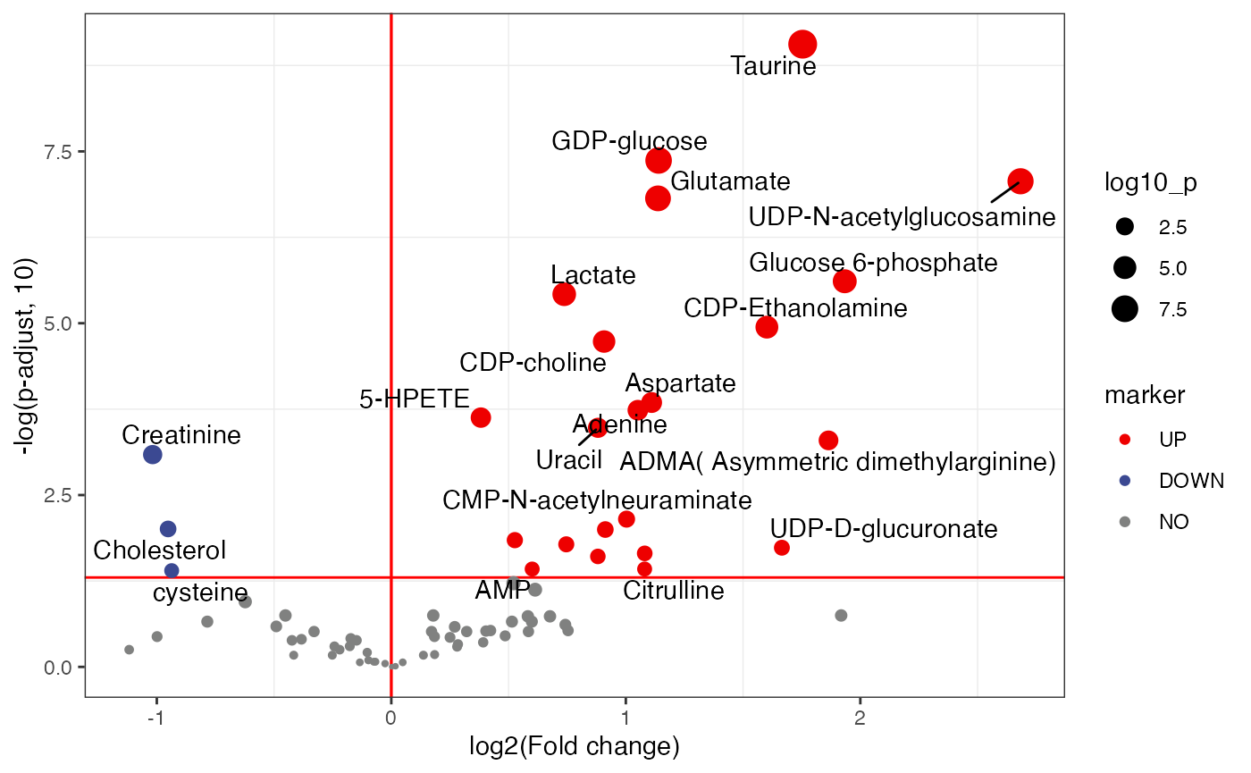
ggsave(plot, filename = "statistical_analysis/male_LCC_vs_male_control.pdf", width = 8, height = 7)
diff_metabolites_malelcc_vs_malecontrol <-
object %>%
activate_mass_dataset(what = "variable_info") %>%
filter(p_value_adjust_malelcc_vs_malecontrol < 0.05) %>%
extract_variable_info()
readr::write_csv(diff_metabolites_malelcc_vs_malecontrol,
file = "statistical_analysis/differential_metabolites.csv")
diff_metabolites_femalelcc_vs_femalecontrol <-
object %>%
activate_mass_dataset(what = "variable_info") %>%
filter(p_value_adjust_femalelcc_vs_femalecontrol < 0.05) %>%
extract_variable_info()
readr::write_csv(diff_metabolites_femalelcc_vs_femalecontrol,
file = "statistical_analysis/differential_metabolites.csv")Heatmap
temp_object <-
object %>%
activate_mass_dataset(what = "sample_info") %>%
filter(sample_id %in% c(malecontrol, maleLCC)) %>%
activate_mass_dataset(what = "variable_info") %>%
filter(variable_id %in% diff_metabolites_malelcc_vs_malecontrol$variable_id) %>%
`+`(1) %>%
log(2) %>%
scale()
library(ComplexHeatmap)
h1 <- HeatmapAnnotation(class = extract_sample_info(temp_object)$group)
massstat::Heatmap(matrix = temp_object,
name = "z-score",
row_names_gp = gpar(cex = 0.4),
column_names_gp = gpar(cex = 0.2),
top_annotation = h1,
row_labels = extract_variable_info(temp_object)$Compound.name,
border = TRUE)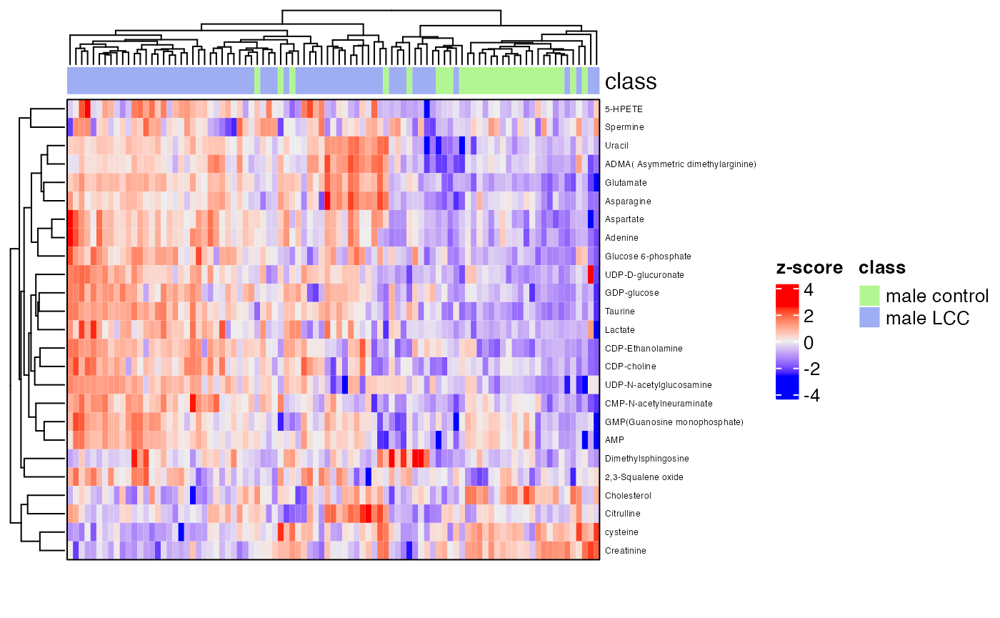
temp_object <-
object %>%
activate_mass_dataset(what = "sample_info") %>%
filter(sample_id %in% c(femalecontrol, femaleLCC)) %>%
activate_mass_dataset(what = "variable_info") %>%
filter(variable_id %in% diff_metabolites_femalelcc_vs_femalecontrol$variable_id) %>%
`+`(1) %>%
log(2) %>%
scale()
library(ComplexHeatmap)
h1 <- HeatmapAnnotation(class = extract_sample_info(temp_object)$group)
massstat::Heatmap(matrix = temp_object,
name = "z-score",
row_names_gp = gpar(cex = 0.4),
column_names_gp = gpar(cex = 0.2),
top_annotation = h1,
row_labels = extract_variable_info(temp_object)$Compound.name,
border = TRUE)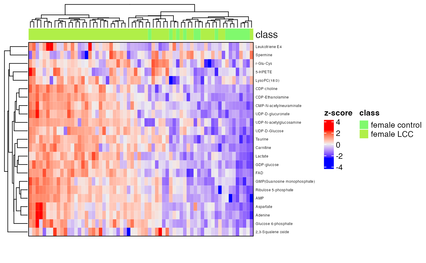
Pathway enrichment analysis
Next, we want to know what pathways are enriched for male and female LCC tumor, respectively.
Load KEGG human pathway database
data("kegg_hsa_pathway", package = "metpath")Remove the disease pathways
#get the class of pathways
pathway_class <-
metpath::pathway_class(kegg_hsa_pathway)
pathway_database <-
kegg_hsa_pathway[remain_idx]Pathway enrichment
kegg_id <-
diff_metabolites_femalelcc_vs_femalecontrol$KEGG.ID
kegg_id <-
kegg_id[!is.na(kegg_id)]
result_female <-
enrich_kegg(query_id = kegg_id,
query_type = "compound",
id_type = "KEGG",
pathway_database = pathway_database,
p_cutoff = 0.05,
p_adjust_method = "BH",
threads = 3)
#> 191 pathways.
save(result_female, file = "pathway_enrichment/result_female")
kegg_id <-
diff_metabolites_malelcc_vs_malecontrol$KEGG.ID
kegg_id <-
kegg_id[!is.na(kegg_id)]
result_male <-
enrich_kegg(query_id = kegg_id,
query_type = "compound",
id_type = "KEGG",
pathway_database = pathway_database,
p_cutoff = 0.05,
p_adjust_method = "BH",
threads = 3)
#> 191 pathways.
save(result_male, file = "pathway_enrichment/result_male")
plot <-
enrich_bar_plot(object = result_male,
x_axis = "p_value",
cutoff = 0.05)
plot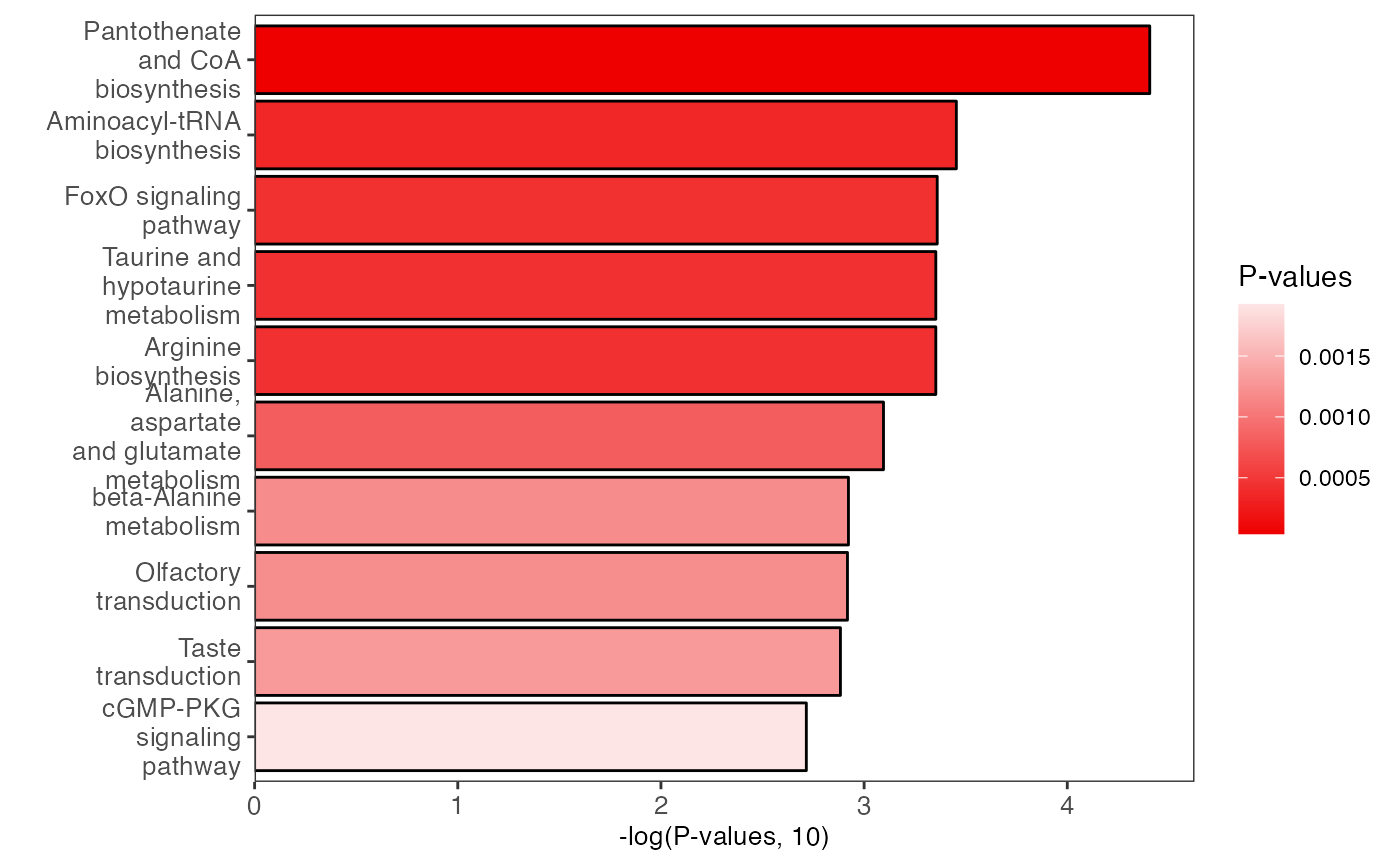
ggsave(plot,
filename = "pathway_enrichment/male_pathway_bar.pdf",
width = 7,
height = 7)
plot <-
enrich_scatter_plot(object = result_male,
y_axis = "p_value",
y_axis_cutoff = 0.05)
plot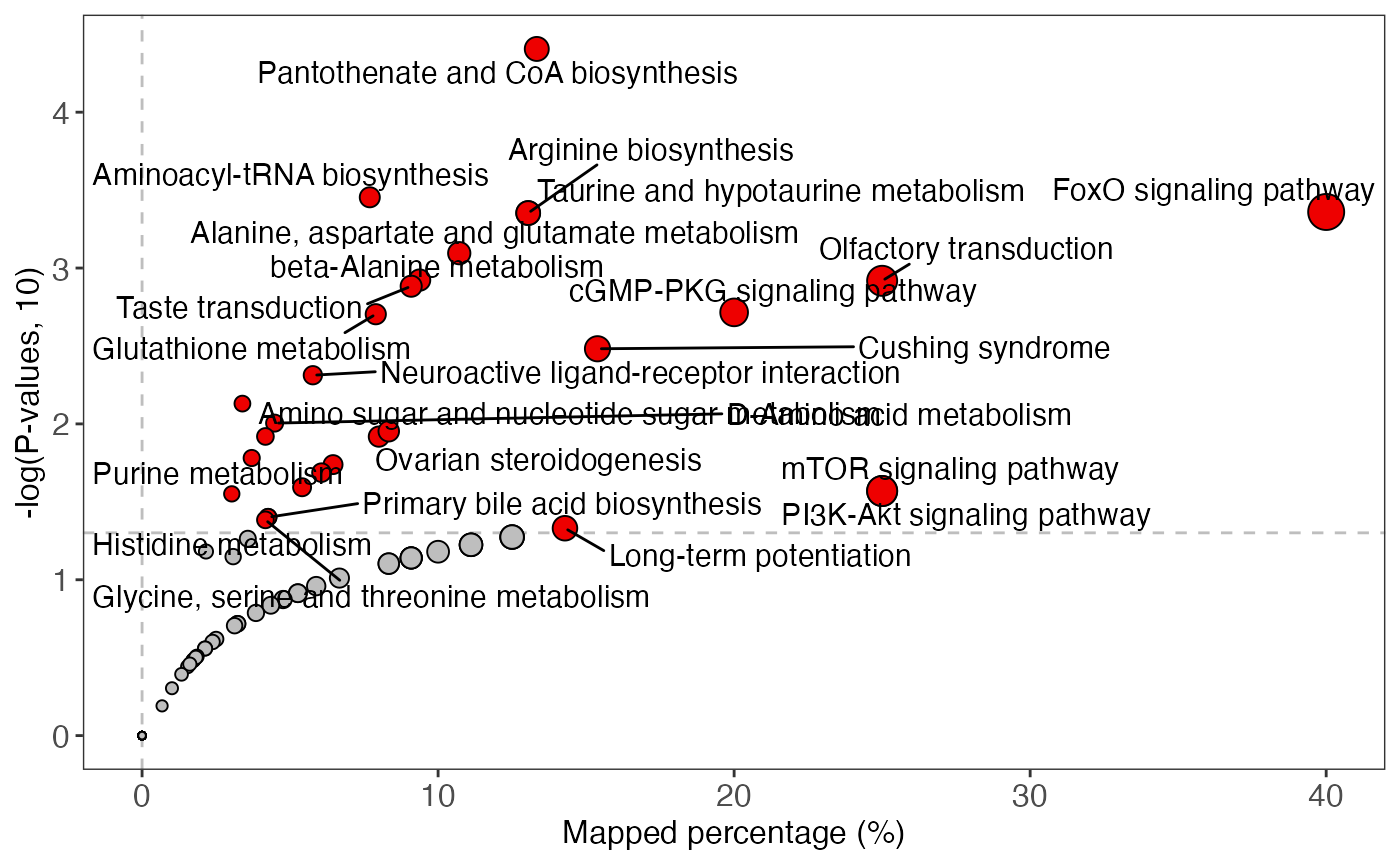
ggsave(plot,
filename = "pathway_enrichment/male_pathway_scatter.pdf",
width = 7,
height = 7)
plot <-
enrich_bar_plot(object = result_female,
x_axis = "p_value",
cutoff = 0.05)
plot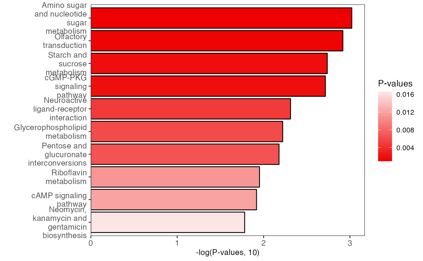
ggsave(plot,
filename = "pathway_enrichment/female_pathway_bar.pdf",
width = 7,
height = 7)
plot <-
enrich_scatter_plot(object = result_female,
y_axis = "p_value",
y_axis_cutoff = 0.05)
plot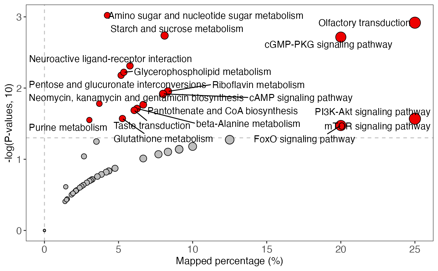
ggsave(plot,
filename = "pathway_enrichment/female_pathway_scatter.pdf",
width = 7,
height = 7)Correlation network analysis
Next, we want to know if the correlation network are different between male and female tumor tissues.
Female tumor
temp_object <-
object %>%
activate_mass_dataset(what = "sample_info") %>%
filter(sample_id %in% c(femalecontrol)) %>%
activate_mass_dataset(what = "variable_info") %>%
filter(variable_id %in% diff_metabolites_femalelcc_vs_femalecontrol$variable_id) %>%
`+`(1) %>%
log(2) %>%
scale()
library(ggraph)
library(tidygraph)
graph_data_female <-
convert_mass_dataset2graph(
object = temp_object,
margin = "variable",
cor_method = "spearman",
p_adjust_cutoff = 1,
p_value_cutoff = 0.05,
pos_cor_cutoff = 0,
neg_cor_cutoff = 0
) %>%
mutate(Degree = centrality_degree(mode = 'all'))
library(extrafont)
loadfonts()
plot <-
ggraph(graph = graph_data_female, layout = "kk") +
geom_edge_fan(aes(color = correlation,
width = -log(p_value, 10)),
show.legend = TRUE) +
geom_node_point(aes(size = Degree)) +
shadowtext::geom_shadowtext(aes(x = x, y = y,
label = Compound.name),
bg.colour = "white",
colour = "black")+
theme_graph() +
scale_edge_color_gradient2(low = "darkblue", mid = "white", high = "red")
plot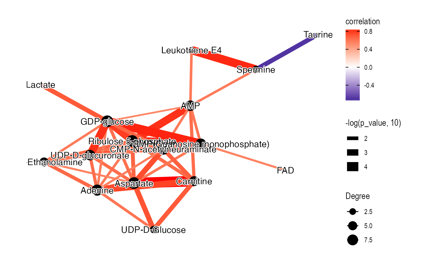
ggsave(plot, filename = "pathway_enrichment/female_cor_network.pdf", width = 7, height = 7)Male tumor
temp_object <-
object %>%
activate_mass_dataset(what = "sample_info") %>%
filter(sample_id %in% c(malecontrol)) %>%
activate_mass_dataset(what = "variable_info") %>%
filter(variable_id %in% diff_metabolites_malelcc_vs_malecontrol$variable_id) %>%
`+`(1) %>%
log(2) %>%
scale()
graph_data_male <-
convert_mass_dataset2graph(
object = temp_object,
margin = "variable",
cor_method = "spearman",
p_adjust_cutoff = 1,
p_value_cutoff = 0.05,
pos_cor_cutoff = 0,
neg_cor_cutoff = 0
) %>%
mutate(Degree = centrality_degree(mode = 'all'))
plot <-
ggraph(graph = graph_data_male, layout = "kk") +
geom_edge_fan(aes(color = correlation,
width = -log(p_value, 10)),
show.legend = TRUE) +
geom_node_point(aes(size = Degree)) +
shadowtext::geom_shadowtext(aes(x = x, y = y,
label = Compound.name),
bg.colour = "white",
colour = "black")+
theme_graph() +
scale_edge_color_gradient2(low = "darkblue", mid = "white", high = "red")
plot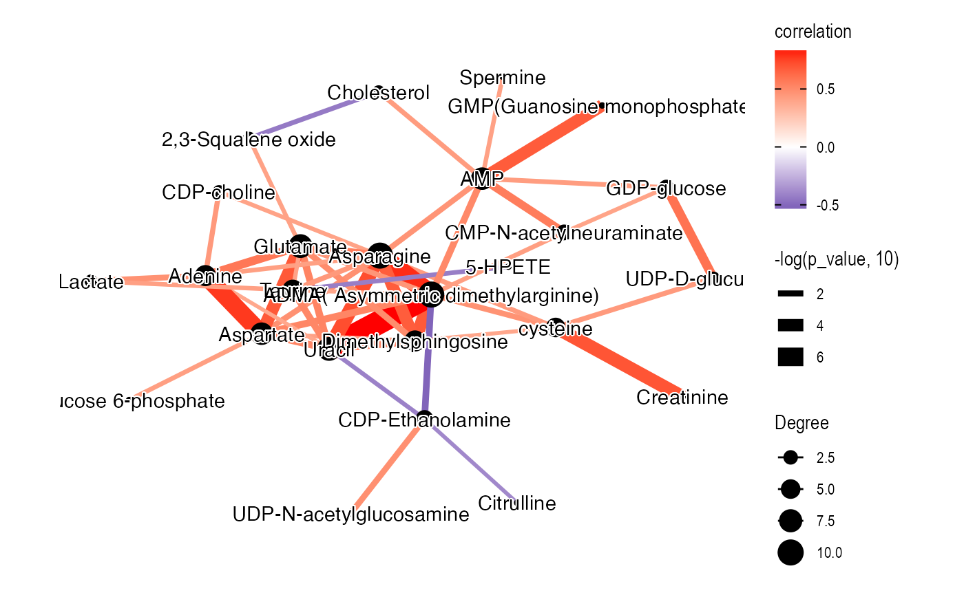
ggsave(plot, filename = "pathway_enrichment/male_cor_network.pdf", width = 7, height = 7)Session information
sessionInfo()
#> R version 4.1.2 (2021-11-01)
#> Platform: x86_64-apple-darwin17.0 (64-bit)
#> Running under: macOS Big Sur 10.16
#>
#> Matrix products: default
#> BLAS: /Library/Frameworks/R.framework/Versions/4.1/Resources/lib/libRblas.0.dylib
#> LAPACK: /Library/Frameworks/R.framework/Versions/4.1/Resources/lib/libRlapack.dylib
#>
#> locale:
#> [1] en_US.UTF-8/en_US.UTF-8/en_US.UTF-8/C/en_US.UTF-8/en_US.UTF-8
#>
#> attached base packages:
#> [1] stats4 grid stats graphics grDevices utils datasets
#> [8] methods base
#>
#> other attached packages:
#> [1] metid_1.2.4 metpath_0.99.4 massstat_0.99.13
#> [4] ggfortify_0.4.14 massqc_0.99.7 masscleaner_0.99.7
#> [7] xcms_3.16.1 MSnbase_2.20.4 ProtGenerics_1.26.0
#> [10] S4Vectors_0.32.3 mzR_2.28.0 Rcpp_1.0.8
#> [13] Biobase_2.54.0 BiocGenerics_0.40.0 BiocParallel_1.28.3
#> [16] massprocesser_0.99.3 magrittr_2.0.2 masstools_0.99.5
#> [19] massdataset_0.99.20 tidymass_0.99.6 shadowtext_0.1.1
#> [22] extrafont_0.17 tidygraph_1.2.0 ggraph_2.0.5
#> [25] ComplexHeatmap_2.10.0 BiocManager_1.30.16 forcats_0.5.1.9000
#> [28] stringr_1.4.0 dplyr_1.0.8 purrr_0.3.4
#> [31] readr_2.1.2 tidyr_1.2.0 tibble_3.1.6
#> [34] ggplot2_3.3.5 tidyverse_1.3.1 remotes_2.4.2
#>
#> loaded via a namespace (and not attached):
#> [1] ragg_1.2.1 bit64_4.0.5
#> [3] missForest_1.4 knitr_1.37
#> [5] DelayedArray_0.20.0 data.table_1.14.2
#> [7] rpart_4.1.16 KEGGREST_1.34.0
#> [9] RCurl_1.98-1.5 doParallel_1.0.17
#> [11] generics_0.1.2 snow_0.4-4
#> [13] leaflet_2.1.0 preprocessCore_1.56.0
#> [15] mixOmics_6.18.1 RANN_2.6.1
#> [17] future_1.23.0 proxy_0.4-26
#> [19] bit_4.0.4 tzdb_0.2.0
#> [21] xml2_1.3.3 lubridate_1.8.0
#> [23] ggsci_2.9 SummarizedExperiment_1.24.0
#> [25] assertthat_0.2.1 viridis_0.6.2
#> [27] xfun_0.29 hms_1.1.1
#> [29] jquerylib_0.1.4 evaluate_0.15
#> [31] DEoptimR_1.0-10 fansi_1.0.2
#> [33] dbplyr_2.1.1 readxl_1.3.1
#> [35] igraph_1.2.11 DBI_1.1.2
#> [37] htmlwidgets_1.5.4 MsFeatures_1.3.0
#> [39] rARPACK_0.11-0 ellipsis_0.3.2
#> [41] RSpectra_0.16-0 crosstalk_1.2.0
#> [43] backports_1.4.1 ggcorrplot_0.1.3
#> [45] MatrixGenerics_1.6.0 vctrs_0.3.8
#> [47] cachem_1.0.6 withr_2.4.3
#> [49] ggforce_0.3.3 itertools_0.1-3
#> [51] robustbase_0.93-9 vroom_1.5.7
#> [53] checkmate_2.0.0 cluster_2.1.2
#> [55] lazyeval_0.2.2 crayon_1.5.0
#> [57] ellipse_0.4.2 labeling_0.4.2
#> [59] pkgconfig_2.0.3 tweenr_1.0.2
#> [61] GenomeInfoDb_1.30.0 nnet_7.3-17
#> [63] globals_0.14.0 rlang_1.0.1
#> [65] lifecycle_1.0.1 affyio_1.64.0
#> [67] extrafontdb_1.0 fastDummies_1.6.3
#> [69] MassSpecWavelet_1.60.0 modelr_0.1.8
#> [71] cellranger_1.1.0 randomForest_4.7-1
#> [73] rprojroot_2.0.2 polyclip_1.10-0
#> [75] matrixStats_0.61.0 Matrix_1.4-0
#> [77] reprex_2.0.1 base64enc_0.1-3
#> [79] GlobalOptions_0.1.2 png_0.1-7
#> [81] viridisLite_0.4.0 rjson_0.2.21
#> [83] clisymbols_1.2.0 bitops_1.0-7
#> [85] pander_0.6.4 Biostrings_2.62.0
#> [87] shape_1.4.6 parallelly_1.30.0
#> [89] robust_0.7-0 jpeg_0.1-9
#> [91] gridGraphics_0.5-1 scales_1.1.1
#> [93] memoise_2.0.1 plyr_1.8.6
#> [95] zlibbioc_1.40.0 compiler_4.1.2
#> [97] RColorBrewer_1.1-2 pcaMethods_1.86.0
#> [99] clue_0.3-60 rrcov_1.6-2
#> [101] cli_3.2.0 affy_1.72.0
#> [103] XVector_0.34.0 listenv_0.8.0
#> [105] patchwork_1.1.1 pbapply_1.5-0
#> [107] htmlTable_2.4.0 Formula_1.2-4
#> [109] MASS_7.3-55 tidyselect_1.1.1
#> [111] vsn_3.62.0 stringi_1.7.6
#> [113] textshaping_0.3.6 highr_0.9
#> [115] yaml_2.3.4 latticeExtra_0.6-29
#> [117] MALDIquant_1.21 ggrepel_0.9.1
#> [119] sass_0.4.0 tools_4.1.2
#> [121] parallel_4.1.2 circlize_0.4.14
#> [123] rstudioapi_0.13 MsCoreUtils_1.6.0
#> [125] foreach_1.5.2 foreign_0.8-82
#> [127] gridExtra_2.3 farver_2.1.0
#> [129] mzID_1.32.0 rvcheck_0.2.1
#> [131] digest_0.6.29 GenomicRanges_1.46.1
#> [133] broom_0.7.12 ncdf4_1.19
#> [135] httr_1.4.2 colorspace_2.0-2
#> [137] rvest_1.0.2 XML_3.99-0.8
#> [139] fs_1.5.2 IRanges_2.28.0
#> [141] splines_4.1.2 yulab.utils_0.0.4
#> [143] pkgdown_2.0.2 graphlayouts_0.8.0
#> [145] ggplotify_0.1.0 plotly_4.10.0
#> [147] systemfonts_1.0.3 fit.models_0.64
#> [149] jsonlite_1.7.3 corpcor_1.6.10
#> [151] R6_2.5.1 Hmisc_4.6-0
#> [153] pillar_1.7.0 htmltools_0.5.2
#> [155] glue_1.6.1 fastmap_1.1.0
#> [157] class_7.3-20 codetools_0.2-18
#> [159] furrr_0.2.3 pcaPP_1.9-74
#> [161] mvtnorm_1.1-3 utf8_1.2.2
#> [163] lattice_0.20-45 bslib_0.3.1
#> [165] magick_2.7.3 zip_2.2.0
#> [167] openxlsx_4.2.5 Rttf2pt1_1.3.9
#> [169] survival_3.2-13 limma_3.50.0
#> [171] rmarkdown_2.11 desc_1.4.0
#> [173] munsell_0.5.0 e1071_1.7-9
#> [175] GetoptLong_1.0.5 GenomeInfoDbData_1.2.7
#> [177] iterators_1.0.14 impute_1.68.0
#> [179] reshape2_1.4.4 haven_2.4.3
#> [181] gtable_0.3.0