Skip to contents

Data preparation

Download the demo data and refer this article.

We have positive and negative mode. For each mode, we have control, case and QC groups. Control group have 110 samples, and case group have 110 samples as well.

Positive mode

massprocesser package is used to do the raw data processing. Please refer this website.

Code

The code used to do raw data processing.

library(tidymass)
#> Registered S3 method overwritten by 'Hmisc':
#>   method       from      
#>   vcov.default fit.models
#> ── Attaching packages ─────────────────────────────────────── tidymass 0.99.4 ──
#>  masscleaner 0.99.3      metid       1.2.2 
#>  massqc      0.99.3      dplyr       1.0.8 
#>  massstat    0.99.6      ggplot2     3.3.5 
#>  metpath     0.99.2
#> ── Conflicts ─────────────────────────────────────────── tidymass_conflicts() ──
#> x massdataset::apply()            masks base::apply()
#> x dplyr::collect()                masks xcms::collect()
#> x massdataset::colMeans()         masks BiocGenerics::colMeans(), base::colMeans()
#> x massdataset::colSums()          masks BiocGenerics::colSums(), base::colSums()
#> x dplyr::combine()                masks MSnbase::combine(), Biobase::combine(), BiocGenerics::combine()
#> x dplyr::filter()                 masks metpath::filter(), massdataset::filter(), stats::filter()
#> x dplyr::first()                  masks S4Vectors::first()
#> x tinytools::get_compound_class() masks masstools::get_compound_class()
#> x tinytools::get_os()             masks masstools::get_os()
#> x tinytools::getDP()              masks masstools::getDP()
#> x dplyr::groups()                 masks xcms::groups()
#> x massdataset::intersect()        masks S4Vectors::intersect(), BiocGenerics::intersect(), base::intersect()
#> x tinytools::keep_one()           masks masstools::keep_one()
#> x dplyr::lag()                    masks stats::lag()
#> x tinytools::ms2_plot()           masks masstools::ms2_plot()
#> x tinytools::ms2Match()           masks masstools::ms2Match()
#> x tinytools::mz_rt_match()        masks masstools::mz_rt_match(), massdataset::mz_rt_match()
#> x tinytools::name_duplicated()    masks masstools::name_duplicated()
#> x metid::read_mgf()               masks tinytools::read_mgf(), masstools::read_mgf()
#> x tinytools::removeNoise()        masks masstools::removeNoise()
#> x dplyr::rename()                 masks massdataset::rename(), S4Vectors::rename()
#> x massdataset::rowMeans()         masks BiocGenerics::rowMeans(), base::rowMeans()
#> x massdataset::rowSums()          masks BiocGenerics::rowSums(), base::rowSums()
#> x tinytools::setwd_project()      masks masstools::setwd_project()
#> x tinytools::split_formula()      masks masstools::split_formula()
#> x tinytools::trans_ID()           masks masstools::trans_ID()
#> x tinytools::trans_id_database()  masks masstools::trans_id_database()
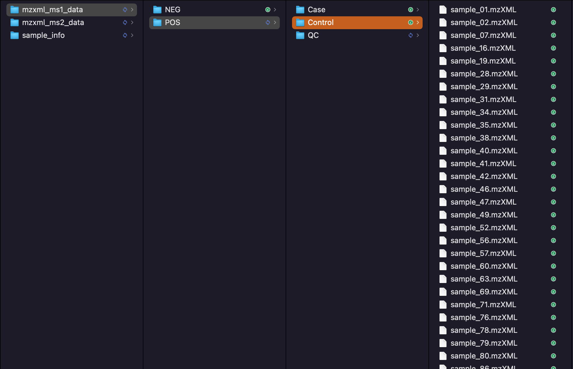
process_data(
  path = "mzxml_ms1_data/POS",
  polarity = "positive",
  ppm = 10,
  peakwidth = c(10, 60),
  threads = 4,
  output_tic = FALSE,
  output_bpc = FALSE,
  output_rt_correction_plot = FALSE,
  min_fraction = 0.5,
  group_for_figure = "QC"
)
#> Reading raw data, it will take a while...
#> 
#> Use old saved data in Result.
#> 
#> ✔ OK
#> 
#> Detecting peaks...
#> 
#> Use old saved data in Result.
#> 
#> ✔ OK
#> 
#> Correcting rentention time...
#>  
#> Use old saved data in Result.
#> 
#> ✔ OK
#> 
#> Grouping peaks across samples...
#> 
#> Use old saved data in Result.
#> 
#> ✔ OK
#> 
#> Outputting peak table...
#> 
#> ✔ OK
#> 
#> OK
#> 
#> ✔ All done!
#> 

Results

All the results will be placed in the folder mzxml_ms1_data/POS/Result. More information can be found here.

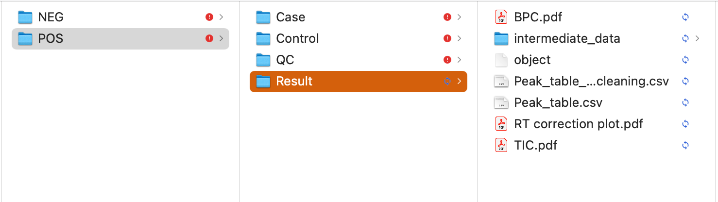
You can just load the object, which is a mass_dataset class object.

load("mzxml_ms1_data/POS/Result/object")
object
#> -------------------- 
#> massdataset version: 0.99.8 
#> -------------------- 
#> 1.expression_data:[ 10149 x 259 data.frame]
#> 2.sample_info:[ 259 x 4 data.frame]
#> 3.variable_info:[ 10149 x 3 data.frame]
#> 4.sample_info_note:[ 4 x 2 data.frame]
#> 5.variable_info_note:[ 3 x 2 data.frame]
#> 6.ms2_data:[ 0 variables x 0 MS2 spectra]
#> -------------------- 
#> Processing information (extract_process_info())
#> create_mass_dataset ---------- 
#>       Package         Function.used                Time
#> 1 massdataset create_mass_dataset() 2022-02-22 16:37:06
#> process_data ---------- 
#>         Package Function.used                Time
#> 1 massprocesser  process_data 2022-02-22 16:36:42

We can see that there are 10,149 metabolic features in positive mode.

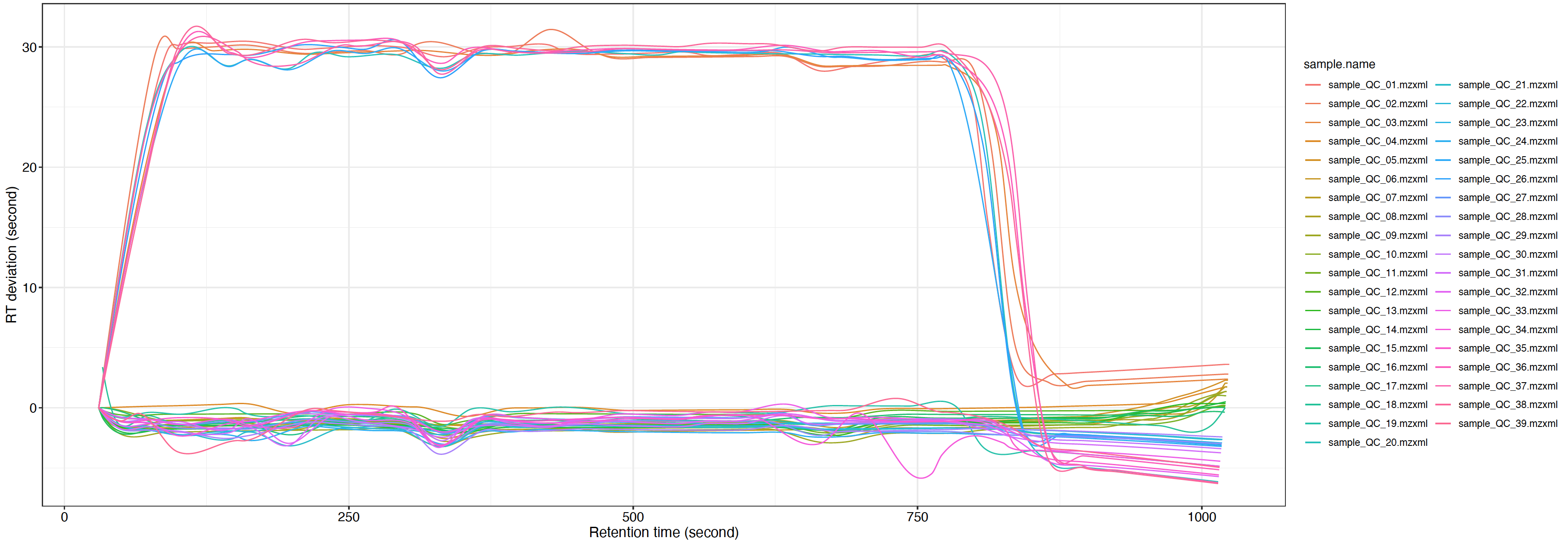
You can use the plot_adjusted_rt() function to get the interactive plot.

load("mzxml_ms1_data/POS/Result/intermediate_data/xdata2")
##set the group_for_figure if you want to show specific groups. And set it as "all" if you want to show all samples.
plot = 
massprocesser::plot_adjusted_rt(object = xdata2, 
                 group_for_figure = "QC", 
                 interactive = TRUE)
plot

Negative mode

The processing of negative mode is same with positive mode data.

Code

Same with positive mode, change polarity to negative.

massprocesser::process_data(
  path = "mzxml_ms1_data/NEG",
  polarity = "negative",
  ppm = 10,
  peakwidth = c(10, 60),
  threads = 4,
  output_tic = FALSE,
  output_bpc = FALSE,
  output_rt_correction_plot = FALSE,
  min_fraction = 0.5,
  group_for_figure = "QC"
)
#> Reading raw data, it will take a while...
#> 
#> Use old saved data in Result.
#> 
#> ✔ OK
#> 
#> Detecting peaks...
#> 
#> Use old saved data in Result.
#> 
#> ✔ OK
#> 
#> Correcting rentention time...
#>  
#> Use old saved data in Result.
#> 
#> ✔ OK
#> 
#> Grouping peaks across samples...
#> 
#> Use old saved data in Result.
#> 
#> ✔ OK
#> 
#> Outputting peak table...
#> 
#> ✔ OK
#> 
#> OK
#> 
#> ✔ All done!
#> 

Results

Same with positive mode.

load("mzxml_ms1_data/NEG/Result/object")
object
#> -------------------- 
#> massdataset version: 0.99.1 
#> -------------------- 
#> 1.expression_data:[ 8804 x 259 data.frame]
#> 2.sample_info:[ 259 x 4 data.frame]
#> 3.variable_info:[ 8804 x 3 data.frame]
#> 4.sample_info_note:[ 4 x 2 data.frame]
#> 5.variable_info_note:[ 3 x 2 data.frame]
#> 6.ms2_data:[ 0 variables x 0 MS2 spectra]
#> -------------------- 
#> Processing information (extract_process_info())
#> create_mass_dataset ---------- 
#>       Package         Function.used                Time
#> 1 massdataset create_mass_dataset() 2022-01-16 16:20:02
#> process_data ---------- 
#>         Package Function.used                Time
#> 1 massprocesser  process_data 2022-01-16 16:19:48

We can see that there are 8,804 metabolic features in negative mode.

Session information

sessionInfo()
#> R Under development (unstable) (2022-01-11 r81473)
#> Platform: x86_64-apple-darwin17.0 (64-bit)
#> Running under: macOS Big Sur/Monterey 10.16
#> 
#> Matrix products: default
#> BLAS:   /Library/Frameworks/R.framework/Versions/4.2/Resources/lib/libRblas.0.dylib
#> LAPACK: /Library/Frameworks/R.framework/Versions/4.2/Resources/lib/libRlapack.dylib
#> 
#> locale:
#> [1] en_US.UTF-8/en_US.UTF-8/en_US.UTF-8/C/en_US.UTF-8/en_US.UTF-8
#> 
#> attached base packages:
#> [1] stats4    stats     graphics  grDevices utils     datasets  methods  
#> [8] base     
#> 
#> other attached packages:
#>  [1] magrittr_2.0.1       tinytools_0.9.1      massdataset_0.99.1  
#>  [4] xcms_3.17.1          MSnbase_2.21.3       ProtGenerics_1.27.2 
#>  [7] S4Vectors_0.33.10    mzR_2.29.1           Rcpp_1.0.7          
#> [10] Biobase_2.55.0       BiocGenerics_0.41.2  BiocParallel_1.29.10
#> [13] massprocesser_0.9.2 
#> 
#> loaded via a namespace (and not attached):
#>   [1] circlize_0.4.14             readxl_1.3.1               
#>   [3] backports_1.4.1             systemfonts_1.0.3          
#>   [5] plyr_1.8.6                  lazyeval_0.2.2             
#>   [7] crosstalk_1.2.0             leaflet_2.0.4.1            
#>   [9] GenomeInfoDb_1.31.1         ggplot2_3.3.5              
#>  [11] digest_0.6.29               yulab.utils_0.0.4          
#>  [13] foreach_1.5.1               htmltools_0.5.2            
#>  [15] fansi_1.0.0                 memoise_2.0.1              
#>  [17] cluster_2.1.2               doParallel_1.0.16          
#>  [19] openxlsx_4.2.5              tzdb_0.2.0                 
#>  [21] limma_3.51.2                ComplexHeatmap_2.11.0      
#>  [23] readr_2.1.1                 modelr_0.1.8               
#>  [25] matrixStats_0.61.0          vroom_1.5.7                
#>  [27] MsFeatures_1.3.0            pkgdown_2.0.1              
#>  [29] colorspace_2.0-2            rvest_1.0.2                
#>  [31] textshaping_0.3.6           haven_2.4.3                
#>  [33] xfun_0.29                   dplyr_1.0.7                
#>  [35] crayon_1.4.2                RCurl_1.98-1.5             
#>  [37] jsonlite_1.7.2              impute_1.69.0              
#>  [39] iterators_1.0.13            glue_1.6.0                 
#>  [41] gtable_0.3.0                zlibbioc_1.41.0            
#>  [43] XVector_0.35.0              GetoptLong_1.0.5           
#>  [45] DelayedArray_0.21.2         shape_1.4.6                
#>  [47] DEoptimR_1.0-10             scales_1.1.1               
#>  [49] vsn_3.63.0                  DBI_1.1.2                  
#>  [51] viridisLite_0.4.0           clue_0.3-60                
#>  [53] gridGraphics_0.5-1          bit_4.0.4                  
#>  [55] preprocessCore_1.57.0       clisymbols_1.2.0           
#>  [57] MsCoreUtils_1.7.1           htmlwidgets_1.5.4          
#>  [59] httr_1.4.2                  RColorBrewer_1.1-2         
#>  [61] ellipsis_0.3.2              farver_2.1.0               
#>  [63] pkgconfig_2.0.3             XML_3.99-0.8               
#>  [65] sass_0.4.0                  dbplyr_2.1.1               
#>  [67] utf8_1.2.2                  labeling_0.4.2             
#>  [69] ggplotify_0.1.0             tidyselect_1.1.1           
#>  [71] rlang_0.4.12                munsell_0.5.0              
#>  [73] cellranger_1.1.0            tools_4.2.0                
#>  [75] cachem_1.0.6                cli_3.1.0                  
#>  [77] generics_0.1.1              broom_0.7.11               
#>  [79] evaluate_0.14               stringr_1.4.0              
#>  [81] fastmap_1.1.0               mzID_1.33.0                
#>  [83] yaml_2.2.1                  ragg_1.2.1                 
#>  [85] bit64_4.0.5                 knitr_1.37                 
#>  [87] fs_1.5.2                    zip_2.2.0                  
#>  [89] robustbase_0.93-8           purrr_0.3.4                
#>  [91] RANN_2.6.1                  ncdf4_1.17                 
#>  [93] pbapply_1.5-0               xml2_1.3.3                 
#>  [95] compiler_4.2.0              rstudioapi_0.13            
#>  [97] plotly_4.10.0               png_0.1-7                  
#>  [99] affyio_1.65.0               reprex_2.0.1               
#> [101] MassSpecWavelet_1.61.0      tibble_3.1.6               
#> [103] bslib_0.3.1                 stringi_1.7.6              
#> [105] desc_1.4.0                  forcats_0.5.1              
#> [107] lattice_0.20-45             Matrix_1.4-0               
#> [109] ggsci_2.9                   vctrs_0.3.8                
#> [111] pillar_1.6.4                lifecycle_1.0.1            
#> [113] BiocManager_1.30.16         GlobalOptions_0.1.2        
#> [115] jquerylib_0.1.4             MALDIquant_1.21            
#> [117] data.table_1.14.2           bitops_1.0-7               
#> [119] GenomicRanges_1.47.6        R6_2.5.1                   
#> [121] pcaMethods_1.87.0           affy_1.73.0                
#> [123] IRanges_2.29.1              codetools_0.2-18           
#> [125] MASS_7.3-55                 assertthat_0.2.1           
#> [127] SummarizedExperiment_1.25.3 rjson_0.2.21               
#> [129] rprojroot_2.0.2             withr_2.4.3                
#> [131] GenomeInfoDbData_1.2.7      parallel_4.2.0             
#> [133] hms_1.1.1                   grid_4.2.0                 
#> [135] tidyverse_1.3.1             tidyr_1.1.4                
#> [137] rmarkdown_2.11              MatrixGenerics_1.7.0       
#> [139] lubridate_1.8.0