Explore data
Xiaotao Shen (https://www.shenxt.info/)
Created on 2021-12-04 and updated on 2022-03-21
explore_data.RmdData preparation
After the raw data processing, peak tables for positive and negative mode have been generated.
Next, we need to get the peak table and sample information and organize them as mass_dataset class objects.
library(tidymass)
#> Registered S3 method overwritten by 'Hmisc':
#>   method       from
#>   vcov.default fit.models
#> ── Attaching packages ─────────────────────────────────────── tidymass 0.99.4 ──
#> ✓ massprocesser 0.99.3     ✓ massstat      0.99.6
#> ✓ masscleaner   0.99.3     ✓ metpath       0.99.2
#> ✓ massqc        0.99.3     ✓ metid         1.2.2
#> ── Conflicts ─────────────────────────────────────────── tidymass_conflicts() ──
#> x massdataset::apply()            masks base::apply()
#> x xcms::collect()                 masks dplyr::collect()
#> x BiocGenerics::colMeans()        masks massdataset::colMeans(), base::colMeans()
#> x BiocGenerics::colSums()         masks massdataset::colSums(), base::colSums()
#> x MSnbase::combine()              masks Biobase::combine(), BiocGenerics::combine(), dplyr::combine()
#> x tidyr::extract()                masks magrittr::extract()
#> x metpath::filter()               masks dplyr::filter(), massdataset::filter(), stats::filter()
#> x S4Vectors::first()              masks dplyr::first()
#> x tinytools::get_compound_class() masks masstools::get_compound_class()
#> x tinytools::get_os()             masks masstools::get_os()
#> x tinytools::getDP()              masks masstools::getDP()
#> x xcms::groups()                  masks dplyr::groups()
#> x S4Vectors::intersect()          masks BiocGenerics::intersect(), massdataset::intersect(), base::intersect()
#> x tinytools::keep_one()           masks masstools::keep_one()
#> x dplyr::lag()                    masks stats::lag()
#> x tinytools::ms2_plot()           masks masstools::ms2_plot()
#> x tinytools::ms2Match()           masks masstools::ms2Match()
#> x tinytools::mz_rt_match()        masks masstools::mz_rt_match(), massdataset::mz_rt_match()
#> x tinytools::name_duplicated()    masks masstools::name_duplicated()
#> x metid::read_mgf()               masks tinytools::read_mgf(), masstools::read_mgf()
#> x MSnbase::reduce()               masks purrr::reduce()
#> x tinytools::removeNoise()        masks masstools::removeNoise()
#> x S4Vectors::rename()             masks dplyr::rename(), massdataset::rename()
#> x BiocGenerics::rowMeans()        masks massdataset::rowMeans(), base::rowMeans()
#> x BiocGenerics::rowSums()         masks massdataset::rowSums(), base::rowSums()
#> x purrr::set_names()              masks magrittr::set_names()
#> x tinytools::setwd_project()      masks masstools::setwd_project()
#> x tinytools::split_formula()      masks masstools::split_formula()
#> x tinytools::trans_ID()           masks masstools::trans_ID()
#> x tinytools::trans_id_database()  masks masstools::trans_id_database()
library(tidyverse)
Positive mode
Load object.
load("mzxml_ms1_data/POS/Result/object")
object_pos <- object
object_pos
#> --------------------
#> massdataset version: 0.99.8
#> --------------------
#> 1.expression_data:[ 10149 x 259 data.frame]
#> 2.sample_info:[ 259 x 4 data.frame]
#> 3.variable_info:[ 10149 x 3 data.frame]
#> 4.sample_info_note:[ 4 x 2 data.frame]
#> 5.variable_info_note:[ 3 x 2 data.frame]
#> 6.ms2_data:[ 0 variables x 0 MS2 spectra]
#> --------------------
#> Processing information (extract_process_info())
#> create_mass_dataset ----------
#>       Package         Function.used                Time
#> 1 massdataset create_mass_dataset() 2022-02-22 16:37:06
#> process_data ----------
#>         Package Function.used                Time
#> 1 massprocesser  process_data 2022-02-22 16:36:42
Read sample information.
sample_info_pos <- readr::read_csv("sample_info/sample_info_pos.csv")
#> Rows: 259 Columns: 6
#> ── Column specification ────────────────────────────────────────────────────────
#> Delimiter: ","
#> chr (4): sample_id, class, subject_id, group
#> dbl (2): injection.order, batch
#>
#> ℹ Use `spec()` to retrieve the full column specification for this data.
#> ℹ Specify the column types or set `show_col_types = FALSE` to quiet this message.
head(sample_info_pos)
#> # A tibble: 6 × 6
#>   sample_id    injection.order class   batch subject_id  group
#>   <chr>                  <dbl> <chr>   <dbl> <chr>       <chr>
#> 1 sample_QC_01               1 QC          1 NA          QC
#> 2 sample_01                  2 Subject     1 subject_474 Control
#> 3 sample_02                  3 Subject     1 subject_431 Control
#> 4 sample_06                  4 Subject     1 subject_414 Case
#> 5 sample_07                  5 Subject     1 subject_830 Control
#> 6 sample_11                  6 Subject     1 subject_125 Case
Add sample_info_pos to object_pos
object_pos %>%
  extract_sample_info() %>%
  head()
#>    sample_id group   class injection.order
#> 1  sample_06  Case Subject               1
#> 2 sample_103  Case Subject               2
#> 3  sample_11  Case Subject               3
#> 4 sample_112  Case Subject               4
#> 5 sample_117  Case Subject               5
#> 6  sample_12  Case Subject               6

object_pos <-
  object_pos %>%
  activate_mass_dataset(what = "sample_info") %>%
  dplyr::select(-c("group", "class", "injection.order"))
object_pos =
  object_pos %>%
  activate_mass_dataset(what = "sample_info") %>%
  left_join(sample_info_pos,
            by = "sample_id")

object_pos %>%
  extract_sample_info() %>%
  head()
#>    sample_id injection.order   class batch  subject_id group
#> 1  sample_06               4 Subject     1 subject_414  Case
#> 2 sample_103              71 Subject     1 subject_330  Case
#> 3  sample_11               6 Subject     1 subject_125  Case
#> 4 sample_112              78 Subject     1 subject_295  Case
#> 5 sample_117              80 Subject     1 subject_793  Case
#> 6  sample_12               8 Subject     1 subject_387  Case
Save the object_pos in a new folder named as data_cleaning.
dir.create("data_cleaning/POS", showWarnings = FALSE, recursive = TRUE)
save(object_pos, file = "data_cleaning/POS/object_pos")
object_pos
#> --------------------
#> massdataset version: 0.99.1
#> --------------------
#> 1.expression_data:[ 10149 x 259 data.frame]
#> 2.sample_info:[ 259 x 6 data.frame]
#> 3.variable_info:[ 10149 x 3 data.frame]
#> 4.sample_info_note:[ 1 x 2 data.frame]
#> 5.variable_info_note:[ 3 x 2 data.frame]
#> 6.ms2_data:[ 0 variables x 0 MS2 spectra]
#> --------------------
#> Processing information (extract_process_info())
#> create_mass_dataset ----------
#>       Package         Function.used                Time
#> 1 massdataset create_mass_dataset() 2022-01-16 16:19:04
#> process_data ----------
#>         Package Function.used                Time
#> 1 massprocesser  process_data 2022-01-16 16:18:43
dim(object_pos)
#> [1] 10149   259
object_pos %>%
  activate_mass_dataset(what = "sample_info") %>%
  dplyr::count(class)
#>     class   n
#> 1      QC  39
#> 2 Subject 220

object_pos %>%
  activate_mass_dataset(what = "sample_info") %>%
  dplyr::count(group)
#>     group   n
#> 1    Case 110
#> 2 Control 110
#> 3      QC  39

object_pos %>%
  activate_mass_dataset(what = "sample_info") %>%
  dplyr::count(batch)
#>   batch   n
#> 1     1 112
#> 2     2 147
So for positive mode, we have 259 samples and 10,149 variables. 220 subject samples and 39 QC samples. 110 control samples and 110 case samples. Two batches in total, 112 samples in batch 1 and 147 in batch 2.
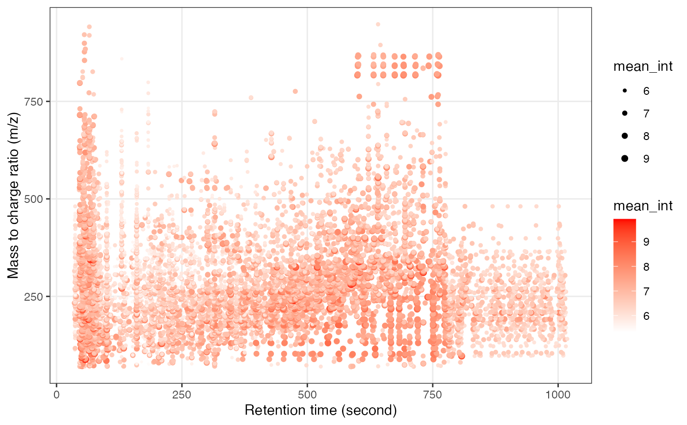
Next, we can get the peak distributation plot of positive mode.
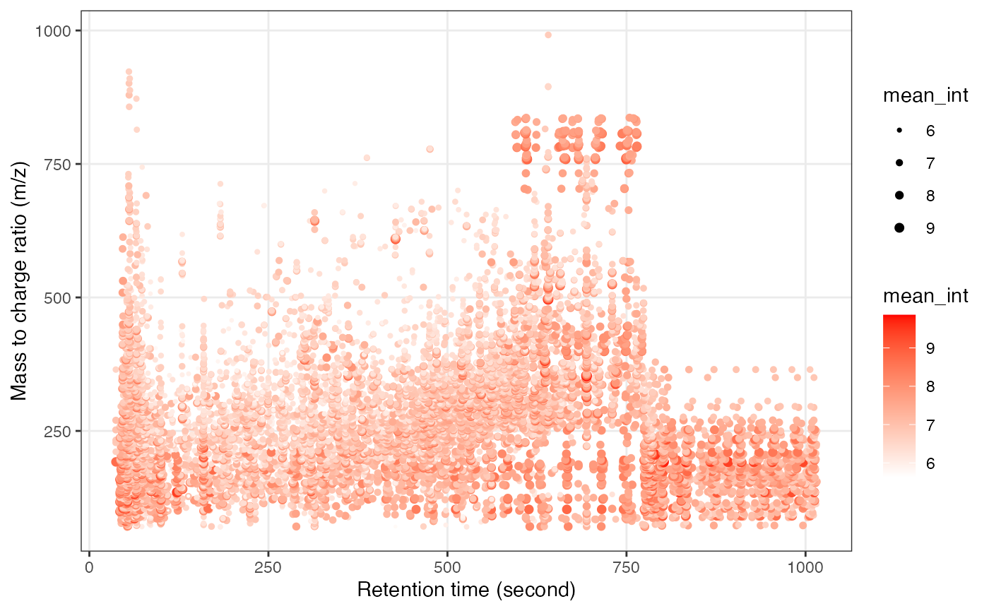
We can explore the missing values (mvs) in positive mode data.
get_mv_number(object = object_pos)
#> [1] 785821
785,821 mvs in total.
get_mv_number(object = object_pos, by = "sample") %>%
  head()
#>  sample_06 sample_103  sample_11 sample_112 sample_117  sample_12
#>       4016       2711       4063       2981       2919       3844
Missing value number in each sample.
get_mv_number(object = object_pos, by = "variable") %>%
  head()
#>  M70T73_POS  M70T53_POS M70T183_POS M70T527_POS M71T695_POS M71T183_POS
#>         129          16         155          54         133         169
Missing value number in each variable.
We can use the figure to show the missing value information.
show_missing_values(object = object_pos, show_column_names = FALSE, percentage = TRUE)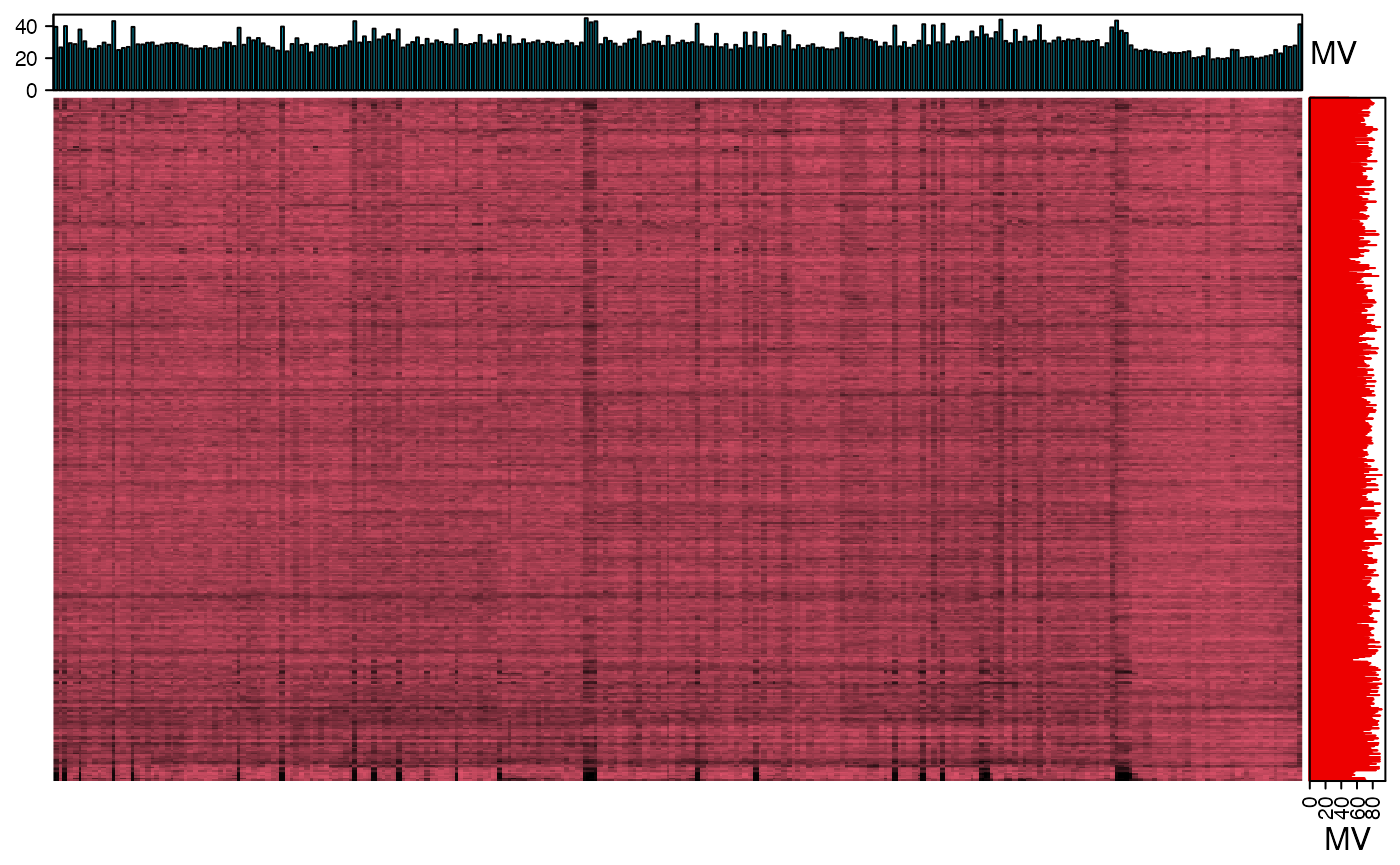
Show the mvs in samples.
show_sample_missing_values(object = object_pos, percentage = TRUE)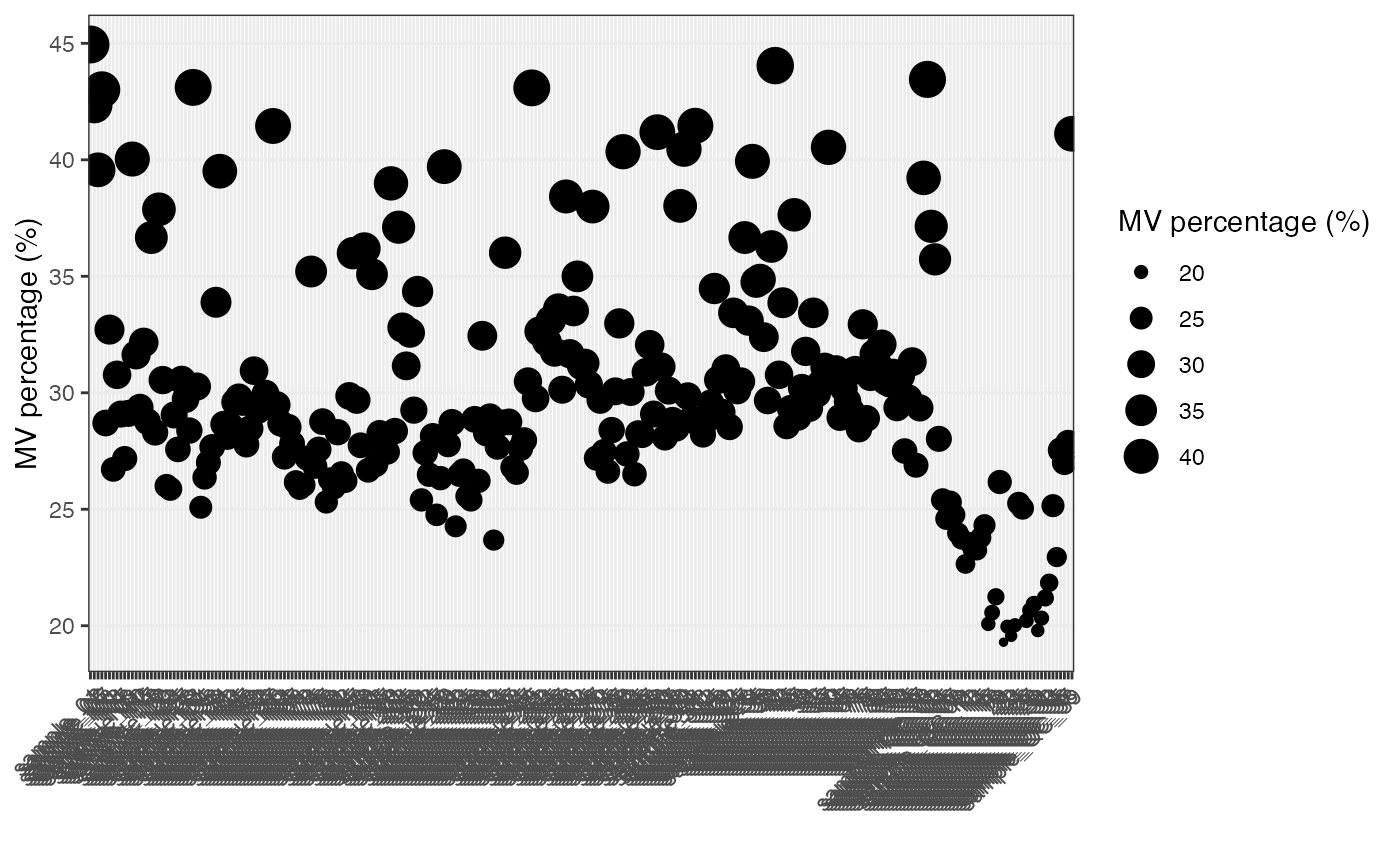
Show the mvs in variables
show_variable_missing_values(
  object = object_pos,
  percentage = TRUE,
  show_x_text = FALSE,
  show_x_ticks = FALSE
) +
  scale_size_continuous(range = c(0.01, 1))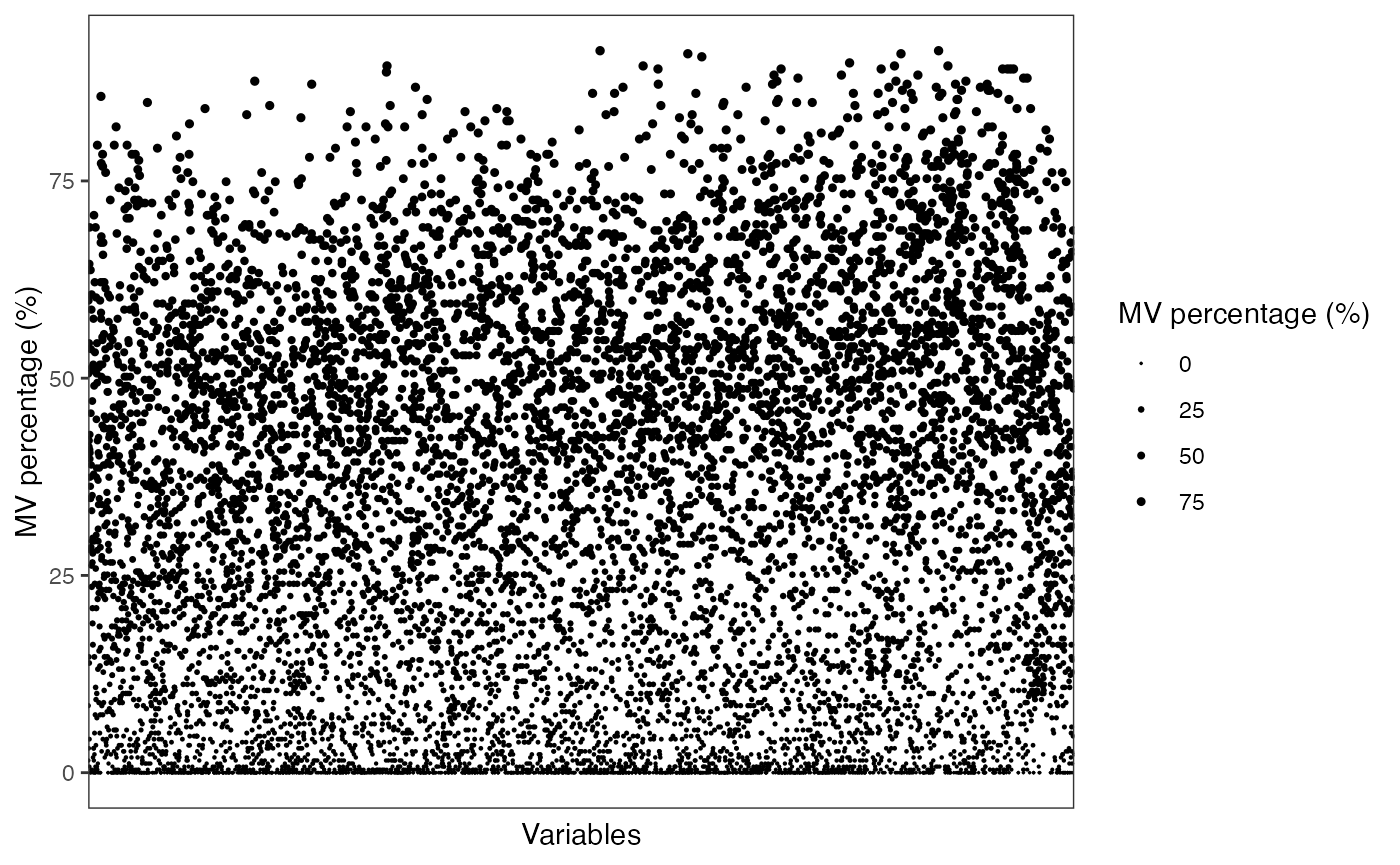
Negative mode
Load object.
load("mzxml_ms1_data/NEG/Result/object")
object_neg <- object
object_neg
#> --------------------
#> massdataset version: 0.99.8
#> --------------------
#> 1.expression_data:[ 8804 x 259 data.frame]
#> 2.sample_info:[ 259 x 4 data.frame]
#> 3.variable_info:[ 8804 x 3 data.frame]
#> 4.sample_info_note:[ 4 x 2 data.frame]
#> 5.variable_info_note:[ 3 x 2 data.frame]
#> 6.ms2_data:[ 0 variables x 0 MS2 spectra]
#> --------------------
#> Processing information (extract_process_info())
#> create_mass_dataset ----------
#>       Package         Function.used                Time
#> 1 massdataset create_mass_dataset() 2022-02-22 16:38:19
#> process_data ----------
#>         Package Function.used                Time
#> 1 massprocesser  process_data 2022-02-22 16:38:02
Read sample information.
sample_info_neg <-
  readr::read_csv("sample_info/sample_info_neg.csv")
#> Rows: 259 Columns: 6
#> ── Column specification ────────────────────────────────────────────────────────
#> Delimiter: ","
#> chr (4): sample_id, class, subject_id, group
#> dbl (2): injection.order, batch
#>
#> ℹ Use `spec()` to retrieve the full column specification for this data.
#> ℹ Specify the column types or set `show_col_types = FALSE` to quiet this message.
head(sample_info_neg)
#> # A tibble: 6 × 6
#>   sample_id    injection.order class   batch subject_id  group
#>   <chr>                  <dbl> <chr>   <dbl> <chr>       <chr>
#> 1 sample_QC_01               1 QC          1 NA          QC
#> 2 sample_01                  2 Subject     1 subject_474 Control
#> 3 sample_02                  3 Subject     1 subject_431 Control
#> 4 sample_06                  4 Subject     1 subject_414 Case
#> 5 sample_07                  5 Subject     1 subject_830 Control
#> 6 sample_11                  6 Subject     1 subject_125 Case
Add sample_info_neg to object_neg
object_neg %>%
  extract_sample_info() %>%
  head()
#>    sample_id group   class injection.order
#> 1  sample_06  Case Subject               1
#> 2 sample_103  Case Subject               2
#> 3  sample_11  Case Subject               3
#> 4 sample_112  Case Subject               4
#> 5 sample_117  Case Subject               5
#> 6  sample_12  Case Subject               6

object_neg <-
  object_neg %>%
  activate_mass_dataset(what = "sample_info") %>%
  dplyr::select(-c("group", "class", "injection.order"))
object_neg <-
  object_neg %>%
  activate_mass_dataset(what = "sample_info") %>%
  left_join(sample_info_neg,
            by = "sample_id")

object_neg %>%
  extract_sample_info() %>%
  head()
#>    sample_id injection.order   class batch  subject_id group
#> 1  sample_06               4 Subject     1 subject_414  Case
#> 2 sample_103              71 Subject     1 subject_330  Case
#> 3  sample_11               6 Subject     1 subject_125  Case
#> 4 sample_112              78 Subject     1 subject_295  Case
#> 5 sample_117              80 Subject     1 subject_793  Case
#> 6  sample_12               8 Subject     1 subject_387  Case
Save the object_neg in a new folder named as data_cleaning.
dir.create("data_cleaning/NEG", showWarnings = FALSE, recursive = TRUE)
save(object_neg, file = "data_cleaning/NEG/object_neg")
object_neg
#> --------------------
#> massdataset version: 0.99.1
#> --------------------
#> 1.expression_data:[ 8804 x 259 data.frame]
#> 2.sample_info:[ 259 x 6 data.frame]
#> 3.variable_info:[ 8804 x 3 data.frame]
#> 4.sample_info_note:[ 1 x 2 data.frame]
#> 5.variable_info_note:[ 3 x 2 data.frame]
#> 6.ms2_data:[ 0 variables x 0 MS2 spectra]
#> --------------------
#> Processing information (extract_process_info())
#> create_mass_dataset ----------
#>       Package         Function.used                Time
#> 1 massdataset create_mass_dataset() 2022-01-16 16:20:02
#> process_data ----------
#>         Package Function.used                Time
#> 1 massprocesser  process_data 2022-01-16 16:19:48
dim(object_neg)
#> [1] 8804  259
object_neg %>%
  activate_mass_dataset(what = "sample_info") %>%
  dplyr::count(class)
#>     class   n
#> 1      QC  39
#> 2 Subject 220

object_neg %>%
  activate_mass_dataset(what = "sample_info") %>%
  dplyr::count(group)
#>     group   n
#> 1    Case 110
#> 2 Control 110
#> 3      QC  39

object_neg %>%
  activate_mass_dataset(what = "sample_info") %>%
  dplyr::count(batch)
#>   batch   n
#> 1     1  86
#> 2     2 173
So for negative mode, we have 259 samples and 8,804 variables. 220 subject samples and 39 QC samples. 110 control samples and 110 case samples. Two batches in total, 112 samples in batch 1 and 147 in batch 2.
Next, we can get the peak distributation plot of negative mode.
We can explore the missing values in negitive mode data.
get_mv_number(object = object_neg)
#> [1] 748253
748,253 mvs in total.
get_mv_number(object = object_neg, by = "sample") %>%
  head()
#>  sample_06 sample_103  sample_11 sample_112 sample_117  sample_12
#>       3029       2766       3298       3100       2912       3053
Missing value number in each sample.
get_mv_number(object = object_neg, by = "variable") %>%
  head()
#> M70T712_NEG M70T527_NEG M70T587_NEG  M70T47_NEG M71T587_NEG M71T641_NEG
#>          16         137           2         146          41          19
Missing value number in each variable.
We can use the figure to show the missing value information.
show_missing_values(object = object_neg, show_column_names = FALSE, percentage = TRUE)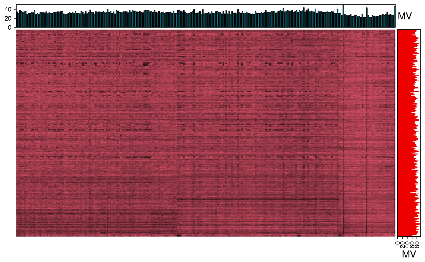
Show the mvs in samples.
show_sample_missing_values(object = object_neg, percentage = TRUE)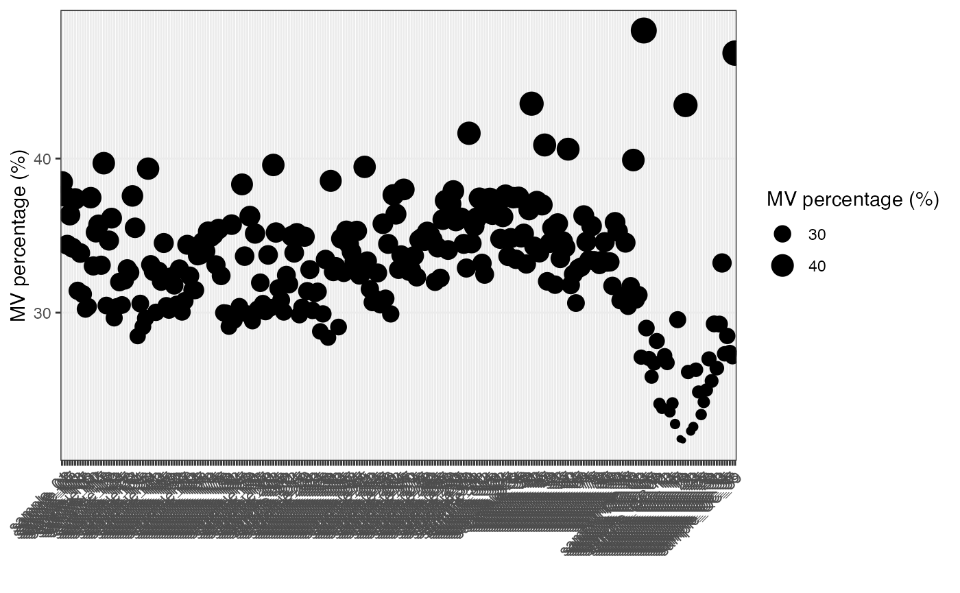
Show the mvs in variables.
show_variable_missing_values(object = object_neg,
                             percentage = TRUE,
                             show_x_text = FALSE,
                             show_x_ticks = FALSE) +
  scale_size_continuous(range = c(0.01, 1))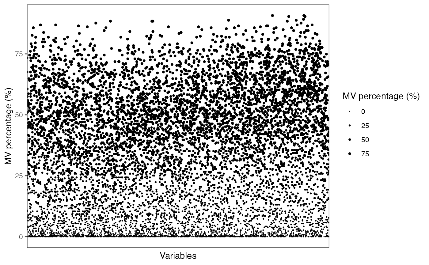
Conclusion
So from those exploration, we have a brief summary of our data. Next, we will use masscleaner pacakge to do the data cleaning of data.
Session information
sessionInfo()
#> R Under development (unstable) (2022-01-11 r81473)
#> Platform: x86_64-apple-darwin17.0 (64-bit)
#> Running under: macOS Big Sur/Monterey 10.16
#>
#> Matrix products: default
#> BLAS:   /Library/Frameworks/R.framework/Versions/4.2/Resources/lib/libRblas.0.dylib
#> LAPACK: /Library/Frameworks/R.framework/Versions/4.2/Resources/lib/libRlapack.dylib
#>
#> locale:
#> [1] en_US.UTF-8/en_US.UTF-8/en_US.UTF-8/C/en_US.UTF-8/en_US.UTF-8
#>
#> attached base packages:
#> [1] stats     graphics  grDevices utils     datasets  methods   base
#>
#> other attached packages:
#>  [1] forcats_0.5.1      stringr_1.4.0      dplyr_1.0.7        purrr_0.3.4
#>  [5] readr_2.1.1        tidyr_1.1.4        tibble_3.1.6       ggplot2_3.3.5
#>  [9] tidyverse_1.3.1    magrittr_2.0.1     tinytools_0.9.1    massdataset_0.99.1
#>
#> loaded via a namespace (and not attached):
#>   [1] matrixStats_0.61.0    fs_1.5.2              bit64_4.0.5
#>   [4] lubridate_1.8.0       doParallel_1.0.16     RColorBrewer_1.1-2
#>   [7] httr_1.4.2            rprojroot_2.0.2       ggsci_2.9
#>  [10] backports_1.4.1       tools_4.2.0           bslib_0.3.1
#>  [13] utf8_1.2.2            R6_2.5.1              DBI_1.1.2
#>  [16] BiocGenerics_0.41.2   lazyeval_0.2.2        colorspace_2.0-2
#>  [19] GetoptLong_1.0.5      withr_2.4.3           tidyselect_1.1.1
#>  [22] leaflet_2.0.4.1       bit_4.0.4             compiler_4.2.0
#>  [25] rvest_1.0.2           textshaping_0.3.6     cli_3.1.0
#>  [28] xml2_1.3.3            desc_1.4.0            plotly_4.10.0
#>  [31] labeling_0.4.2        sass_0.4.0            scales_1.1.1
#>  [34] pbapply_1.5-0         pkgdown_2.0.1         systemfonts_1.0.3
#>  [37] digest_0.6.29         yulab.utils_0.0.4     rmarkdown_2.11
#>  [40] pkgconfig_2.0.3       htmltools_0.5.2       highr_0.9
#>  [43] dbplyr_2.1.1          fastmap_1.1.0         readxl_1.3.1
#>  [46] htmlwidgets_1.5.4     rlang_0.4.12          GlobalOptions_0.1.2
#>  [49] rstudioapi_0.13       farver_2.1.0          shape_1.4.6
#>  [52] gridGraphics_0.5-1    jquerylib_0.1.4       generics_0.1.1
#>  [55] jsonlite_1.7.2        vroom_1.5.7           crosstalk_1.2.0
#>  [58] zip_2.2.0             ggplotify_0.1.0       Rcpp_1.0.7
#>  [61] munsell_0.5.0         S4Vectors_0.33.10     fansi_1.0.0
#>  [64] lifecycle_1.0.1       stringi_1.7.6         yaml_2.2.1
#>  [67] plyr_1.8.6            grid_4.2.0            parallel_4.2.0
#>  [70] crayon_1.4.2          haven_2.4.3           circlize_0.4.14
#>  [73] hms_1.1.1             magick_2.7.2          knitr_1.37
#>  [76] ComplexHeatmap_2.11.0 pillar_1.6.4          rjson_0.2.21
#>  [79] codetools_0.2-18      stats4_4.2.0          reprex_2.0.1
#>  [82] glue_1.6.0            evaluate_0.14         modelr_0.1.8
#>  [85] data.table_1.14.2     tzdb_0.2.0            png_0.1-7
#>  [88] vctrs_0.3.8           foreach_1.5.1         cellranger_1.1.0
#>  [91] gtable_0.3.0          clue_0.3-60           assertthat_0.2.1
#>  [94] cachem_1.0.6          xfun_0.29             openxlsx_4.2.5
#>  [97] broom_0.7.11          ragg_1.2.1            viridisLite_0.4.0
#> [100] iterators_1.0.13      memoise_2.0.1         IRanges_2.29.1
#> [103] cluster_2.1.2         ellipsis_0.3.2