Annotate metabolites according to MS2 database using metid
Xiaotao Shen PhD (https://www.shenxt.info/)
Created on 2020-03-28 and updated on 2022-09-19
Source:vignettes/metabolite_annotation_using_MS2.Rmd
metabolite_annotation_using_MS2.RmdMS1 data preparation
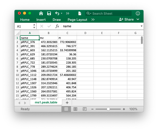
The peak table must contain “name” (peak name), “mz” (mass to charge ratio) and “rt” (retention time, unit is second). It can be from any data processing software (XCMS, MS-DIAL and so on).
MS2 data preparation
The raw MS2 data from DDA or DIA should be transfered to msp, mgf or mzXML format files using ProteoWizard software.
Database
The database must be generated using constructDatabase()
function. You can also use the public databases we provoded here.
Data organization
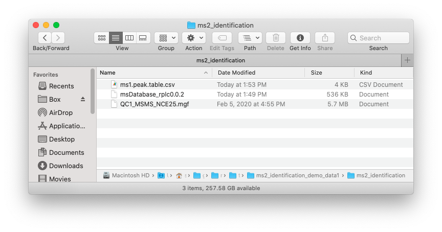
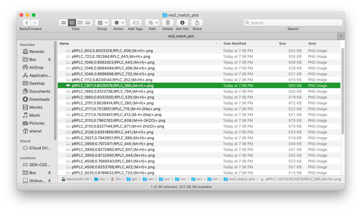
Place the MS1 peak table, MS2 data and database which you want to use in one folder like below figure shows:
Run identify_metabolites()
function
We use the demo data in metid package to show how to use
metid to identify metablite without MS2 spectra. Here, we
use the in-house database from Michael Snyder lab
(snyder_database_rplc0.0.3).
In-house database The in-house database in our lab were provided, with RPLC and HILIC mode RT information. They were acquired using Thermo Fisher QE-plus. However, the LC system may be different with your experiments, so if you want to use our in-house database for metabolite identification, please set
rt.match.tolas 100000000 (no limitation). The in-house database can be downloaded in my github.
Load demo datas
First we load the MS1 peak, MS2 data and database from
metid package and then put them in a example
folder.
#creat a folder nameed as example
path <- file.path(".", "example")
dir.create(path = path, showWarnings = FALSE)

##get MS1 peak table from metid
ms1_peak <- system.file("ms1_peak", package = "metid")
file.copy(from = file.path(ms1_peak, "ms1.peak.table.csv"),
          to = path, overwrite = TRUE, recursive = TRUE)
#> [1] TRUE

##get MS2 data from metid
ms2_data <- system.file("ms2_data", package = "metid")
file.copy(from = file.path(ms2_data, "QC1_MSMS_NCE25.mgf"),
          to = path, overwrite = TRUE, recursive = TRUE)
#> [1] FALSE

##get database from metid
database <- system.file("ms2_database", package = "metid")

data("snyder_database_rplc0.0.3", package = "metid")
save(snyder_database_rplc0.0.3, file = file.path(path, "snyder_database_rplc0.0.3"))
Now in your ./example, there are three files, namely
ms1.peak.table.csv, QC1_MSMS_NCE25.mgf and
snyder_database_rplc0.0.3.
Use m/z, RT and MS2 for metabolite identification
annotate_result3 <-
  identify_metabolites(ms1.data = "ms1.peak.table.csv",
                       ms2.data = c("QC1_MSMS_NCE25.mgf"),
                       ms2.match.tol = 0.5,
                       ce = "all",
                       ms1.match.ppm = 15,
                       rt.match.tol = 30,
                       polarity = "positive",
                       column = "rp",
                       path = path,
                       candidate.num = 3,
                       database = "snyder_database_rplc0.0.3",
                       threads = 3)
#>
  |
  |                                                                      |   0%
  |
  |===                                                                   |   4%
  |
  |======                                                                |   9%
  |
  |=========                                                             |  13%
  |
  |============                                                          |  17%
  |
  |===============                                                       |  22%
  |
  |==================                                                    |  26%
  |
  |=====================                                                 |  30%
  |
  |========================                                              |  35%
  |
  |===========================                                           |  39%
  |
  |==============================                                        |  43%
  |
  |=================================                                     |  48%
  |
  |=====================================                                 |  52%
  |
  |========================================                              |  57%
  |
  |===========================================                           |  61%
  |
  |==============================================                        |  65%
  |
  |=================================================                     |  70%
  |
  |====================================================                  |  74%
  |
  |=======================================================               |  78%
  |
  |==========================================================            |  83%
  |
  |=============================================================         |  87%
  |
  |================================================================      |  91%
  |
  |===================================================================   |  96%
  |
  |======================================================================| 100%
Note: You can also provide more than one MS2 data. Just provide them to
ms2.dataas a vector.
Most of the parameters are same with in
Annotate metabolites according to MS1 database using metid package.
Some parameters for MS2 matching:
ms2.data: The ms2 data.ce: The collision energy of spectra used for matching. Set asallto use all the spectra.ms2.match.tol: The MS2 similarity tolerance for peak and database metabolite match. The MS2 similarity refers to the algorithm from MS-DIAl. So if you want to know more information about it, please read this publication.
\[MS2\;Simlarity\;Score\;(SS) = Fragment\;fraction*Weight_{fraction} + Dot\;product(forward) * Weight_{dp.reverse}+Dot\;product(reverse)*Weight_{dp.reverse}\]
-
fraction.weight: The weight for fragment match fraction.
\[Fragment\;match\;fraction = \dfrac{Match\;fragement\;number}{All\;fragment\;number}\]
dp.forward.weight: The weight for dot product (forward)dp.forward.weight: The weight for dot product (forward)
\[Dot\;product = \dfrac{\sum(wA_{act.}wA_{lib})^2}{\sum(wA_{act.})^2\sum(wA_{lib})^2}with\;w =1/(1+\dfrac{A}{\sum(A-0.5)})\]
The return result annotate_result3 is a
metIdentifyClass object, you can directory get the brief
information by print it in console:
annotate_result3Get detailed annotation information
Most of the detailed annotation information are same with
Annotate metabolites according to MS1 database using metid package.
Get MS2 spectra match plot
You can also use ms2plot() function to output the MS2
specra match plot for one, multiple or all peaks.
Output one MS2 spectra match plot.
##which peaks have identifications
which_has_identification(annotate_result3) %>%
  head()
#>   MS1.peak.name               MS2.spectra.name
#> 1     pRPLC_603 mz162.112442157672rt37.9743312
#> 2     pRPLC_722  mz181.072050304971rt226.14144
#> 3    pRPLC_1046 mz181.072050673093rt196.800648
#> 4    pRPLC_1112 mz209.092155077047rt58.3735608
#> 5    pRPLC_1307 mz314.232707486156rt400.268664
#> 6    pRPLC_1860   mz249.185015539689rt579.6807
Becase we need the information from database, so we need to load database first.
ms2.plot1 <- ms2plot(object = annotate_result3,
                     database = snyder_database_rplc0.0.3,
                     which.peak = "pRPLC_603")
ms2.plot1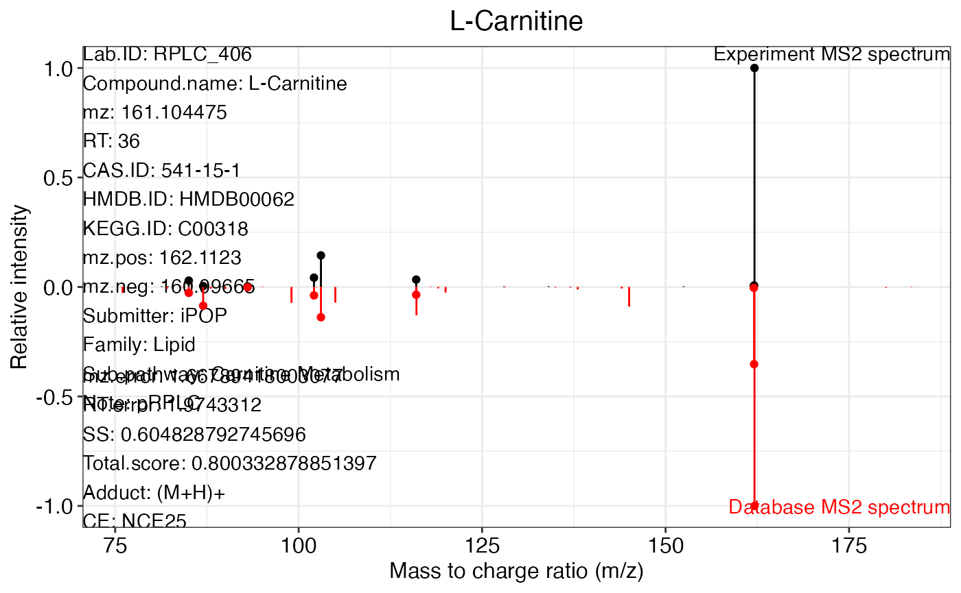
You can also output interactive MS2 spectra match plot by setting
interaction.plotas TRUE.
##which peaks have identification
ms2.plot2 <- ms2plot(object = annotate_result3,
                     database = snyder_database_rplc0.0.3,
                     which.peak = "pRPLC_603",
                     interaction.plot = TRUE)
ms2.plot2
Some time you want to get the dark theme. Because the plot from
ms2plot is a ggplot2 object, so you can just
set the theme as ‘dark theme’.
ms2.plot1 <- ms2plot(object = annotate_result3,
                     database = snyder_database_rplc0.0.3,
                     which.peak = "pRPLC_603",
                     col.exp = "white")
ms2.plot1_2 <-
  ms2.plot1 +
  ggdark::dark_theme_bw()

ms2.plot1_2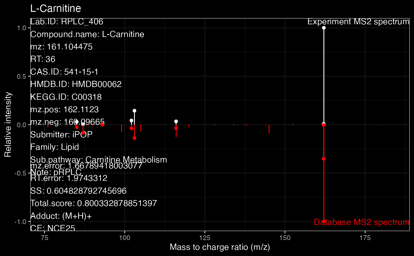
Just use plotly to convert it to interactive plot.
Output multiple or all MS2 spectra match plots
You can set the which.peak as a vector of peak names to
output multiple peaks MS2 match plot, or set it as all to
output all MS2 spectra match plots.
For example, if we want to output all the MS2 spectra match plots:
ms2plot(
  object = annotate_result3,
  database = snyder_database_rplc0.0.3,
  which.peak = "all",
  path = file.path(path, "inhouse"),
  threads = 3
)
Then all the MS2 spectra match plots will be output in the “inhouse” folder.
Session information
sessionInfo()
#> R version 4.2.1 (2022-06-23)
#> Platform: x86_64-apple-darwin17.0 (64-bit)
#> Running under: macOS Big Sur ... 10.16
#>
#> Matrix products: default
#> BLAS:   /Library/Frameworks/R.framework/Versions/4.2/Resources/lib/libRblas.0.dylib
#> LAPACK: /Library/Frameworks/R.framework/Versions/4.2/Resources/lib/libRlapack.dylib
#>
#> locale:
#> [1] en_US.UTF-8/en_US.UTF-8/en_US.UTF-8/C/en_US.UTF-8/en_US.UTF-8
#>
#> attached base packages:
#> [1] stats     graphics  grDevices utils     datasets  methods   base
#>
#> other attached packages:
#>  [1] tinytools_0.9.1    forcats_0.5.1.9000 stringr_1.4.0      dplyr_1.0.9
#>  [5] purrr_0.3.4        readr_2.1.2        tidyr_1.2.0        tibble_3.1.7
#>  [9] tidyverse_1.3.1    ggplot2_3.3.6      massdataset_1.0.5  magrittr_2.0.3
#> [13] masstools_0.99.13  metid_1.2.16
#>
#> loaded via a namespace (and not attached):
#>   [1] backports_1.4.1             readxl_1.4.0
#>   [3] circlize_0.4.15             systemfonts_1.0.4
#>   [5] plyr_1.8.7                  lazyeval_0.2.2
#>   [7] crosstalk_1.2.0             BiocParallel_1.30.3
#>   [9] listenv_0.8.0               GenomeInfoDb_1.32.2
#>  [11] Rdisop_1.56.0               digest_0.6.29
#>  [13] foreach_1.5.2               yulab.utils_0.0.5
#>  [15] htmltools_0.5.2             fansi_1.0.3
#>  [17] memoise_2.0.1               cluster_2.1.3
#>  [19] doParallel_1.0.17           tzdb_0.3.0
#>  [21] openxlsx_4.2.5              limma_3.52.2
#>  [23] ComplexHeatmap_2.12.0       globals_0.15.1
#>  [25] modelr_0.1.8                matrixStats_0.62.0
#>  [27] vroom_1.5.7                 pkgdown_2.0.5
#>  [29] prettyunits_1.1.1           colorspace_2.0-3
#>  [31] rvest_1.0.2                 haven_2.5.0
#>  [33] textshaping_0.3.6           xfun_0.31
#>  [35] crayon_1.5.1                RCurl_1.98-1.7
#>  [37] jsonlite_1.8.0              impute_1.70.0
#>  [39] iterators_1.0.14            glue_1.6.2
#>  [41] gtable_0.3.0                zlibbioc_1.42.0
#>  [43] XVector_0.36.0              GetoptLong_1.0.5
#>  [45] DelayedArray_0.22.0         ggdark_0.2.1
#>  [47] shape_1.4.6                 BiocGenerics_0.42.0
#>  [49] scales_1.2.0                vsn_3.64.0
#>  [51] DBI_1.1.3                   Rcpp_1.0.8.3
#>  [53] mzR_2.30.0                  viridisLite_0.4.0
#>  [55] progress_1.2.2              clue_0.3-61
#>  [57] gridGraphics_0.5-1          bit_4.0.4
#>  [59] preprocessCore_1.58.0       stats4_4.2.1
#>  [61] MsCoreUtils_1.8.0           htmlwidgets_1.5.4
#>  [63] httr_1.4.3                  RColorBrewer_1.1-3
#>  [65] ellipsis_0.3.2              farver_2.1.1
#>  [67] pkgconfig_2.0.3             XML_3.99-0.10
#>  [69] dbplyr_2.2.1                sass_0.4.1
#>  [71] utf8_1.2.2                  labeling_0.4.2
#>  [73] ggplotify_0.1.0             tidyselect_1.1.2
#>  [75] rlang_1.0.3                 munsell_0.5.0
#>  [77] cellranger_1.1.0            tools_4.2.1
#>  [79] cachem_1.0.6                cli_3.3.0
#>  [81] generics_0.1.3              broom_1.0.0
#>  [83] evaluate_0.15               fastmap_1.1.0
#>  [85] mzID_1.34.0                 yaml_2.3.5
#>  [87] ragg_1.2.2                  bit64_4.0.5
#>  [89] knitr_1.39                  fs_1.5.2
#>  [91] zip_2.2.0                   ncdf4_1.19
#>  [93] pbapply_1.5-0               future_1.26.1
#>  [95] xml2_1.3.3                  compiler_4.2.1
#>  [97] rstudioapi_0.13             plotly_4.10.0
#>  [99] png_0.1-7                   affyio_1.66.0
#> [101] reprex_2.0.1                bslib_0.3.1
#> [103] stringi_1.7.6               highr_0.9
#> [105] desc_1.4.1                  MSnbase_2.22.0
#> [107] lattice_0.20-45             ProtGenerics_1.28.0
#> [109] Matrix_1.4-1                ggsci_2.9
#> [111] vctrs_0.4.1                 pillar_1.7.0
#> [113] lifecycle_1.0.1             furrr_0.3.0
#> [115] BiocManager_1.30.18         jquerylib_0.1.4
#> [117] MALDIquant_1.21             GlobalOptions_0.1.2
#> [119] data.table_1.14.2           bitops_1.0-7
#> [121] GenomicRanges_1.48.0        R6_2.5.1
#> [123] pcaMethods_1.88.0           affy_1.74.0
#> [125] IRanges_2.30.0              parallelly_1.32.0
#> [127] codetools_0.2-18            MASS_7.3-57
#> [129] assertthat_0.2.1            SummarizedExperiment_1.26.1
#> [131] rprojroot_2.0.3             rjson_0.2.21
#> [133] withr_2.5.0                 S4Vectors_0.34.0
#> [135] GenomeInfoDbData_1.2.8      parallel_4.2.1
#> [137] hms_1.1.1                   grid_4.2.1
#> [139] rmarkdown_2.14              MatrixGenerics_1.8.1
#> [141] lubridate_1.8.0             Biobase_2.56.0